


The Continuous Time Random Walk and the Finite Difference Method for the Space Time Fractional Diffusion Equations
Abdel-Rehim EA*
Department of Mathematics and Computer Science, Suez Canal University, Egypt
Submission: August 28, 2017; Published: October 13, 2017
*Corresponding author: Abdel-Rehim EA, Department of Mathematics and Computer Science, Faculty of Science, Suez Canal University, Ismailia, Egypt, Email: entsarabdelrehim@yahoo.com, entsarabdelrehim@gmail.com
How to cite this article: Abdel R E. The Continuous Time Random Walk and the Finite Difference Method for the Space Time Fractional Diffusion Equations. Biostat Biometrics Open Acc J. 2017; 3(3): 555615. DOI: 10.19080/BBOAJ.2017.03.555615
Abstract
The space fractional diffusion equations are a linear partial pseudo-differential equation with spatial fractional derivatives in space. This equation arises when the motion of the particle is not Brownian and there are extremely long jumps whose length is distributed according to the Levy long tail Some physical, biological and chemical models exhibit a power law with a non integer frequency of order t-β,0 < β <1. In this case, one needs to replace the first order time differential operator by the Caputo time fractional operator. In this paper, I am interested in finding the approximation solution of the space time fractional diffusion equations by using the common finite difference rules beside using the Gruenwald-Letnikove difference scheme for the fractional differential operators. The approximation solution is proved to be conditionally stable. Finally, some numerical examples are given based on this method
MSC 2010 : Primary 26A33, Secondary 45K05, 60J60, 44A10, 42A38, 60G50, 65N06, 47G30,80-99
Keywords: Diffusion equations; Finite difference; Caputo fractional derivative; Riesz fractional operator; Stationary solutions; Levy stable distribution; Continuous time random walk
Introduction
In 1827 an English botanist, Robert Brown, noticed that small particles suspended in fluids perform peculiarly erratic movements. This phenomenon, which can also be observed in gases, is referred to as Brownian motion [1]. It was not until 1905 that Albert Einstein first advanced a satisfactory theory. Einstein considered the case of the free particle, that is, a particle in which no forces other than those due to the molecules of the surrounding medium are acting. He was able to show that the probability density u(x, t) must satisfy the partial differential equation

where α > 0 is a certain physical constant. This equation is called the diffusion equation or the free diffusion. The conditions imposed on u are

The solution u(x, t) of equation (1.1) with the initial condition u(x, 0) =δ (x-x0) is well known as the corresponding Green function or the fundamental solution. As soon as the theory for the free particle was established, a natural question arose how it should be modified in order to take into account the outside forces F (x), for example, gravity which acts in the direction of the x-axis and forces the particle to go back to the origin. When the external force is proportional to the distance from the origin, it has shown that equation (1.1) should be replaced by

This partial differential equation describes the elastic diffusive motion of a bounded particle (for example, small pendulum) and being a special case of the general (diffusion- convection equation), see [2-4]. equation (1.2) is a special case from Fokker Planck equation which reads

Where

It is well known that the Ehrenfest Model is mathematically modelled by the Fokker Planck equation. The Fokker-Planck equation (FPE ) is one of the most widely used equations of statistical physics for studying the dynamic behaviour of stochastic differential equations driven by Gaussian noises, see [5-7]. However, it turns out that many other physical phenomena are outside this frame work. Especially solutes that move through fractal media commonly exhibits large deviations from the stochastic processes of Brownian motion and do not require finite velocity. The extension to Levy stable motion is a straight forward generalization due to the common properties of Levy stable motion and Brownian motion, but the Levy flights differ from the regular Brownian motion by the occurrence of extremely long jumps whose length is distributed according to the Levy long tail  Many physical, biological, medical, and chemical models exhibits a power law with a non integer frequency of order t-β, where 0 <β<1 for diffusion processes and 0 <β<2 for wave propagation. Also in a complex inhomogeneous conducting medium experimental evidence shows that the sound waves propagate with power law of non integer order. 1 <β<2
Such processes have a memory. In this paper, I give a review about the approximate, analytical and the continuous time random walk of the space time fractional diffusion processes under the action of constant and linear forces. Therefore, this paper is written in 6 sections. Section 1 is devoted to the introduction. Section 2 is to the important used notations. In section 3, I study the continuous time random walk of the space fractional diffusion equations. In section 4, the approximate and reversibility of the time fractional Ehrenfest model are discussed. Sections 5 and 6 are devoted to the explicit and implicit approximate solutions of the diffusion equations under the action of a constant force.
Importent notations
In this research papers, I use the space fractional operator

which is called the Feller space-fractional differentiation operator of order a, where and I adopt the notation introduced by Zaslavsky, who considered it as a power of the positive definitive operator  , see Oldham & Spanier [8], Ross & Miller [9], and recently Gorenflo & Mainardi [10-13]. This form must not be confused with a power of the first order differential operator xD01. The Fourier transform of
xD0α reads.
, see Oldham & Spanier [8], Ross & Miller [9], and recently Gorenflo & Mainardi [10-13]. This form must not be confused with a power of the first order differential operator xD01. The Fourier transform of
xD0α reads.

While

The operator xD0α is expressed as the negative inverse of the suitable integral operator (Riesz potential) I0α whose symbol is  and can be written as

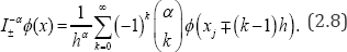
Where I0-α is the inverse of the symmetric Riesz potential. fractional integral operators I0-α is defined as

Where

Therefore, the symmetric Riesz potential can be written as

Where I±α denote the Riemann-Liouville fractional integral operators, by some people called Weyl integrals. Because of equation (5.3), the approximation solution of this equation are studied at α=2,0< α<1,1<α<2,andα=11 separately.
Grünwald-Letnikov Scheme for all Values of
The approximating of xI±-αin the Grunwald-Letnikov scheme for the different values of a is listed below. Firstly for 0<α<1

secondly for 1 <α≤2
Third for α =1 One cannot use the Grunwald-Letnikov discretization of xD0α as α =1 because the denominator equation (5.3). Instead of the Grünwald-Letnikov discretization, I use the discretization used by R. Goreno, who replaced the factor 
Caputo time-fractional derivative
The time fractional derivative operator of order is defined as

being called the memory function, see [14-18]. This kernel enables us to reflect the memory effects of many physical processes. The Laplace transform of it reads
.png "Click here to view Large Figure 1")

The continuous time random walk of the diffusion equations
The space-fractional diffusion equation, [19], reads

This equation has a solution in the Fourier domain, namely

The space fractional diffusion with central linear drift reads

Where α > 0 and b > 0 . This equation has a solution in the Fourier domain as

I use Bilers transformation between the two pairs of the independent variables (x,t) and (ﻉ,t) as

This transformation enables to transfer the solution of the space-fractional diffusion equation to be a solution of the space- fractional Fokker-Planck equation. In [19], I use the Monte Carlo method to simulate the random walk of the discussed model. For this purpose, I generate two random variables (Xn, Tn). First we suppose that a particle starts at the origin (x0 = 0), and waits a period of time Tn, at a particular location (xn-1,Tn) before moving instantaneously to the next location with jump width are iid and likewise the jumps χnare iid. Furthermore the waiting times and the jumps are independent of each other. The new position at ,∀=1,2,....We call Tn the waiting times the new position at tn=tn-1+Tnwhich is equivalent to

and the particle remains resting at x = xn-1 in the time interval tn <t < tn+1. For generating the random variable Xn , i. e. the jump, having the Cauchy or the Gaussian distributions, we use the method of inversion which seems to be simple and most effective. We also use the same method to simulate the random variable T, i. e. the waiting time, having an exponential distribution with mean 1. For simulating the jump X corresponding stable distribution, αϵ(0,2) we use the method given in the book of Janciki [21], in order to simulate the random variable X having a symmetric and nonsymmetric α-stable distribution. Firstly, for the symmetric α - stable random variable X, i. e. β = 0 we follow the steps
a) Generate a random variable V uniformly distributed on -π/2,π/2 and an exponential random variable W with mean 1,
b) Compute

Secondly, for the non-symmetric α stable random variables X with β ϵ[-1,1], one has to follow the following steps
I. Generate a random variable V uniformly distributed -π/2,π/2 on and an exponential random variable W with mean 1,
II. Compute
.png "Click here to view Large Figure 1")
Where


In the numerical result section, I give some numerical results for the jumps of the diffused particles, see Figures [1-4]. The first column represents the CTRW of the diffusion, DE and the second column represents the CTRW of the diffusion under the action of attractive linear force, FPE.
Time fractional Ehrenfest model
The Ehrenfest model, classical case, and the time-fractional Ehrenfest model are considered as stochastic processes and are mathematically modelled by the time-fractional diffusion equation under the action of an attractive linear force, equation (3.4. For more information about the classical Ehrenfest model, see [18]. Equation (3.4) for α = 2 has the solution

Replace the first order time-derivative by Caputo time- fractional derivative of order β, where βϵ(0,1] and replace (Ę, t) by simply(x, t) . One gets

The solution of this equation is getting by using the separation of variables as

Where Eβ(-ntβ) is the Mittag-Le-ffler function and Dn (x) is the Weber function. It is worth to say that in [20], I studied the fundamental solution (Green function) of the space-time fractional Ehrenfest model by replacing  in equation (4.1) by xD0α Applying the discretization of the Caputo time fractional operator being given in equation (2.10) beside the common finite difference rule for descretizing
  and
and  at eqution(4.1) then solving for
 gets
gets

The discrete scheme for the classical case is put in the matrix form

Here i  that pT means is a stochastic matrix and the classical Ehrenfest forms a Markov chain. While the discrete scheme for the time-fractional Ehrenfest model is put in the matrix form

where the matrix Q = qij is defined as

Here i that QT pv That means the matrix QT is not a stochastic matrix and therefore its process is not a Markov chain. Both matrices can be written as

where H is a matrix whose its rows are summed to zero. The elements of the stochastic matrix P converge to the binomial distribution at n->∞as

Where

The stationary row of the matrix Q is getting by using the eigenvector y* with eigenvalue zero of the matrix H. Define y = cy , to be the stationary solution of the matrix Q, where
Convergence of the Discrete Approximate Solution of both Models
Define, first the vector z such that  and the difference vector d (t)= {d (t0), d (t1), d (t2),...},
where

For the Ehrenfest model, d(t)


Where ω and are constants. The stationary probability vectors and are simulated at Figure 5
Definition of the reversibility property
The definition of the reversible process as it is stated at the book of Kelly is as follows: A stochastic process X (t)is said to be reversible if X (t1 ), X (t2) ,...., X (tn) has the same distribution as X (τ-t1) X (τ-t2),...., X X (τ-tn), The balance equation is satisfied for both classical and non classical model where for the classical reads

and for the time-fractional Ehrenfest is

although the classical is Ehrenfest is Markov and the non classical is Non-Markov.
The space-time fractional diffusion under the action of a constant force
The advection dispersion equations, stfade is mathematically models the particle motion at the earth surface. This equation is obtained from equation (1.3) and equation (1.4) by replacing
F (x ) = -b, i.e. by a constant force. Here I study its space-time fractional version which reads

Where 0 <β≤1,0<α≤2,α#1.Here a, and b are positive constants representing the dispersion coefficient and the average fluid velocity respectively. Here tD*β is the Caputo time-fractional operator. I study its space-time fractional version. Namely I investigate its approximate solution by using the explicit finite difference method, see [22]. The Laplace transform of tD*βreads

xD*βis the Riesz space-fractional operator of order which in Fourier domain reads

Riesz Potential: This operator represents the negative inverse of the Riesz Potential I0α whose symbol is  i,e..
i,e..

where the symmetric Riesz Potential operator is defined as

Because of equation (5.3), the approximation solution of this equation are studied at α = 2,0<α<11<α<2 and α< 1 separately. One must distinguish the descretization of hI± with respect to the value of α , as follows:

For α=1, one has to replace the factor  . in equations (5.4) and (5.5) by . for 0k= , and
  �For k=0,and
 for
for  the numerical calculations, one has to join the descretization of equation (5.4) and equation (5.5) with that of tD*βu(x,t)to get the explicit scheme of the space-time fractional advection equation. The descreate
scheme of the space-time fractional advection equation. The descrete scheme of this equation is written in the matrix form
the numerical calculations, one has to join the descretization of equation (5.4) and equation (5.5) with that of tD*βu(x,t)to get the explicit scheme of the space-time fractional advection equation. The descreate
scheme of the space-time fractional advection equation. The descrete scheme of this equation is written in the matrix form

Where


Where  . I have proved in [22] that the discrete schemes of these model converge, in the Fourier-Laplace domain, to the Fourier-Laplace transforms of the Corresponding fractional differential equations for all values of α and β . The bath of the diffused particle y((n))= y (tn) for different values of the time is simulated at Figures [6-8] and . In Figure [9], I simulated the singular case, i.e. as
The space-time fractional diffusion under the action of a constant force
In this section, I study the implicit difference scheme of the advection diffusion equation (5.1), see [23], by using θ- the method which is also known as the weighted method. The idea of the method is to replace y(n)in the right hand side of thesolved equation (5.6) by

The implicit method allows to discuss the path of the diffusion in the long run. Therefore, I have numerically compared at this paper the path of the diffusive particles for large values of t . The stability analysis of the discrete schemes are discussed and proved for each value of α and β according to the Von- Neumann Necessary condition for Stability [24]. I have used here the diffusion and drift constants as variables to adjust the value of R for each values of α and β . Consequently the value of μ is also varied. Finally, to simulate the path of the diffused particle for different values of t,α and β , Figures 10-13


Numerical Result
References
- M Kac (1950) Random walk and the theory of Brownian motion. The American Mathematical Monthly 54(7): 369-391.
- Uhlenbeck GE, Ornstein LE (1930) On the theory of Brownian motion, Physical Review 36(5): 823-841.
- Wang MC, Uhlenbeck GE (1956) On the theory of Brownian motion, Reviews of Modern Physics, 17(2-3): 323-342.
- Smoluchowski, Drei Vortrage uber Di usion (1916) Brownsche molekularbe-wegung und koagulation von kolloidteilchen, Zeitschrift fur Physic 17: 557-571.
- Kolwankar KM, Gangal AD (1998) Local fractional Fokker-Planck equation, Physical Review Letters 80(2): 214-217.
- Metzler R, Barkai E, Klafter J (1998) Anomalous di usion and relaxation close to thermal equiliubrium: a fractional Fokker-Planck equation approach, Phsical Review Letters 82(18): 3563-3567.
- Risken H (1989) The Fokker-Planck equation (methods solution and applica-tions) (2nd edn.), Springer-Verlag, Berlin, Heidelberg, USA.
- Oldham KB, Spanier J (1974) The Fractional Calculus, Vol. 3 of Mathematics in Science and Engineering, Academic Press, New York, USA.
- Miller KS, Ross B (1993) An Introduction to the fractional calculus and fractional differential equations, John Wily and Sons, INC., New York, Chichester, Brisbane, Toronto, Singapore.
- Gorenflo R, Vivoli A (2003) Fully discrete random walks for the space time fractional diffusion equations, Signal Processing 83(2003): 24112420.
- Gorenflo R, Mainardi F (1998) Random walk models for space- fractional diffusion processes, Fractional Calculus and Applied Analysis, 1(2): 167-191.
- Gorenflo R, Mainardi F (1999) Approximation of Levy- Feller diffusion by random walk, J. for Analysis and its Applications (ZAA) 18: 231-146.
- Gorenflo R (1997) Fractional calculus: some numerical methods. Fractals and Fractional Calculus in Continuum Mechanics 378: 277290.
- Gorenflo R, Mainardi F, Moretti D, Paradisi P (2002) Time-Fractional diffusion: a discrete random walk approach. Nonlinear Dynamics, 29(1-4): 129 143.
- Gorenflo R, Abdel-Rehim EA (2005) Discrete models of time-fractional diffusion in a potential well, Fractional Calculus and Applied Analysis 8(2): 173-200.
- Gorenflo R, Abdel-Rehim EA (2007) Convergence of the Grunwald- Letnikov scheme for time-fractional diffusion. Journal of Computational and Applied Mathematics 205(2): 871-881.
- Gorenflo R, Abdel-Rehim EA (2008) Simulation of continuous time ran-dom walk of the space-fractional diffusion equations, Journal of Computational and Applied Mathematics 222: 274-285.
- Abdel-Rehim EA (2009) From the Ehrenfest model to time-fractional stochastic processes. Journal of Computational and Applied Mathematics 233(2): 197-207.
- Gorenflo R, Abdel-Rehim EA (2008) Simulation of continuous time random walk of the space-fractional diffusion equations, Journal of Computational and Applied Mathematics 222(2): 274-283.
- Abdel-Rehim EA (2016) Fundamental solutions of the fractional diffusion and the fractional Fokker-Planck equations, Journal of the Egyptian Mathematical Society 24: 337-347.
- Janicki A (1996) Numerical and statistical approximation of stochastic differential equations with non-gaussian measures, Monograph No. 1, H Steinhaus Center for Stochastic Methods in Science and Technology, Technical University, Worclaw, Poland.
- Abdel-Rehim EA (2013) Explicit approximation solutions and proof of con-vergence of the space time fractional advection dispersion equations, Scientific Research: Journal of Applied Mathematics 4: 1427-1440.
- Abdel-Rehim EA (2015) Implicit difference scheme of the space-time frac-tional advection diffusion equation, Journal of fractional calculus & Ap-plied Analysis, 18(6): 1252-1276.
- Lax PD, Richtmyer RD (1956) Survey of the stability of linear finite difference equations, Communication on Pure and Applied Mathematics 9(3): 267-293.


