


Quantile Regression in Biostatistics
Jayabrata Biswas1, Hemant Kulkarni2 and Kiranmoy Das1*
1Interdisciplinary Statistical Research Unit, Indian Statistical Institute, India
2Human Genetics Unit, Indian Statistical Institute, India
Submission: May 11, 2017; Published: August 17, 2017
*Corresponding author: Kiranmoy Das, Interdisciplinary Statistical Research Unit, Indian Statistical Institute, India; Email: kiranmoy.das@gmail.com
How to cite this article: Jayabrata B, Hemant K, Kiranmoy D. Quantile Regression in Biostatistics. Biostat Biometrics Open Acc J. 2017: 2(5): 555596. DOI: 10.19080/BBOAJ.2017.02.555596.
Abstract
Quantile regression has been a very effective modelling approach in many real applications. Unlike the mean regression, quantile regression focuses on modelling the entire distribution of the response variable, not just the mean value. We review some working models of quantile regression. We demonstrate some real applications of such modelling in Biostatistics and related disciplines. We also discuss some recent developments in modelling multiple responses in the context of quantile regression.
Keywords: Asymmetric Laplace Distribution; Linear Model; Mean Regression; Quantile Regression
Introduction
The goal of regression analysis is to find certain summary of response variable for a given set of explanatory variables. Classical regression approach based on Least Squares (LS) method focuses on the conditional mean of the response variable for the given set of covariates. There are certain attractive features of mean regression which make it popular and practically useful. First, the least squares method is easy for computation and interpretation. Second, classical regression assumes Gaussian distribution on noise and homoscedasticity in variance which helps to develop attractive statistical theory for the estimator of model parameters.
Though the mean regression has widely been used in many disciplines, it has a couple of limitations. Assumptions related to random errors are not always satisfied in reality. Regression model gives misleading results in the presence of outliers. Median regression is an alternative method which models median instead of mean for a given set of covariates. The objective function for the mean regression is the error sum of squares while for the median regression it is the sum of the absolute deviations. Median regression performs better in the presence of outliers and hence more robust compared to the mean regression. Though median regression has been proposed for quite a long time, due to the computational issues it has not been as popular as the mean regression.
Both the mean and median regression give the information on the central tendency of the response given the covariates. Both these methods actually give partial information of the response.In order to get complete information on the response variable at the various quantile values we need to go beyond the central tendency. Koenker, et al. [1] introduced the quantile regression model where conditional quantile of response is a linear function of covariates. Quantile regression models response at different levels of quantiles and thus gives the information on the shape of the response distribution. Objective function of quantile regression varies over different levels of quantile and thus leads potentially distinct solutions which can be interpreted as the effect of covariates at the respective quantile level.
Note that the median regression is a special case of quantile regression at the quantile level τ =0.5. Quantile regression uses weighted absolute sum as the objective function which can also be represented using linear programming problem and can be solved by simplex algorithm. Quantile regression model not only gives the complete distributional picture, it has several other advantages over the linear regression method. The objective function of quantile regression makes it more robust in the presence of outliers. Most importantly, no distributional assumption is needed for the response variable in quantile regression.
The robustness of the quantile regression makes it extremely useful in various disciplines. In drug discovery an investigator is interested in studying the effects of certain covariates at the higher values of clinical measurements. In clinical studies, the diagnosis of disease is done based on the range of certain clinical measurements. If these measurements are controlled by certain covariates (e.g. age, gender etc.), then giving different quantile levels of clinical measurement is more informative than giving only the mean. Other than the biomedical discipline quantile regression is also useful in other areas, such as in social studies, a researcher might be interested in evaluating the effect of various covariates at lower (poor) and upper (rich) levels of economic status. In educational studies, school authorities are more interested in finding the factors affecting the exam scores at lower and upper levels.
The current article is organized as the following. In section 2 we discuss quantile regression model, and section 3 focuses on the inference related to model parameter(s). Section 4 illustrates some practical applications of quantile regression in biostatistics. Finally, section 5 concludes.
Model
In the current presentation, we consider the data in the form (XTi, yi), for i = 1, 2, . . . , N, where is a continuous response variable with cumulative distribution functionFy (the exact form Fy of is unknown), and XTi is the P dimensional row vector of the covariates. Then the linear conditional quantile functions are expressed as the following
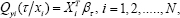
for 0 < τ < 1, Qyi = F-1yi, βτ and is the quantile specific vector of parameters. Note that the above representation can be alternatively written as the following linear model:
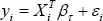
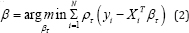
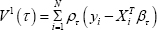
Where the residuals are iid with the τ -th quantile=0. Note that βτ is estimated by minimizing the following objective function:

As discussed earlier, this objective function is represented as a linear programming problem and can be solved by simplex algorithm. Objective function given in (1) is also written in the form of:

where ρτ (u) = u( τ -I(u < 0)) is a loss function and I(.) denotes the indicator function.
Linear regression assumes a normal error distribution and thus the maximum likelihood estimation approach can be used for the parameter estimation. Similarly for the quantile regression one can use Asymmetric Laplace Distribution [ALD] [2,3] for the response and develop a similar maximum likelihood estimation procedure. The joint likelihood function based on the ALD is given as the following:
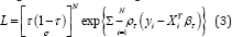
where ρτ is the same check function as in (2), σ > 0 is the scale parameter, while τ ∈ (0, 1) controls the skewness of the distribution. Yu, et al. [4] discuss more properties of ALD. Standard Laplace distribution is special case of ALD at τ = 0.5. By maximizing the above likelihood function, we can obtain the MLE of βτ. However, we note that the distributional assumption here is purely artificial and the ALD model is just a working model. In general, for quantile regression we do not need any distributional assumption.
Inference
In this section we describe certain inference related to the model parameter(s). We start with asymptotic procedure for testing and constructing a confidence interval for parameters. Later we discuss two bootstrap approaches and the goodness of fit procedure.
Asymptotic approach
Similar to standard linear regression model one can also develop asymptotic theory for quantile regression. Under certain regularity condition it can be shown that,
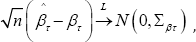
where ∑βτ is the asymptotic variance covariance matrix and is given as:
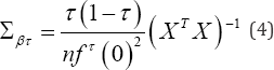
where X is design matrix and fτ (0) is probability density (of ALD) error term evaluated at the τ -th quantile. Since we use ALD as only working model for likelihood procedure, the exact form of residual distribution is unknown. Detail procedure of obtaining residual density given in equation (4) is discussed by Koenkar [5]. From equation (4) it is clear that standard error of parameter depends on the residual distribution. Often due to skewness and outliers, the iid assumption is violated. Thus the asymptotic procedure might give misleading results, alternative approach is to develop distribution free estimation procedure as discussed below.
Bootstrap
Bootstrap is an alternative approach of obtaining the sampling distribution of the param-eters. Bootstrap method based on resampling was proposed by Effron [6]. For the quantile regression, both the design matrix bootstrap and error bootstrap can be performed. In design matrix bootstrap the random samples (y*i,X*i ) are drawn from empirical distribution of (yi,Xi),i = 1,........,N . Usual quantile regression procedure is carried out on this bootstrap sample to obtain estimator β* τ . Repeating this procedure B times yields B such estimator's β*(1)τ,...., β*(B)τ standard error and confidence intervals are obtained using these B estimators.
Error bootstrap approach is carried out by resampling the residuals. Let e* =( e*1,...., e*N) is randomly drawn from the sample residuals. Let defineyi* = XiTβ+ e*i,i= l..... N . Estimator β*i is obtain applying usual quantile regression procedure for y*i Xi. Repeat this procedures B times to get bootstrap distribution and hence standard error and confidence interval. One can also carry out parametric bootstrap approach by assuming ALD as residual distribution. Error bootstrap method gives efficient results under the assumption of independent residuals and violation of this assumption makes the bootstrap method extremely poor.
Goodness of Fit
In linear regression the goodness of fit is measured by R-square which is interpreted as the proportion of variation explained by covariates. This quantity lies between 0 to 1, R2 and closer to 1 indicates better fit. Koenker, et al. [2] propose notion of goodness of fit by replacing squared measures by the weighted absolute measure. Let is weighted distance measured for τ -th quantile regression model and
  is corresponding sample distance measured for null model. Where Q°( τ ) is τ - th quantile of y}, y2, , yn, the goodness of fit measurement is given as:

Interpretation of R ( τ) is similar to the R2 in the classical regression.
Biostatistics applications
Weight and age study: Weight and age data on 4011 US girls were collected (Cole, 1988) to study the relationship between age and weight. Linear regression model is not much effective for this data for a couple of reasons, (i) the data is highly right skewed, (ii) homoscedasticity assumption is not valid because for higher age we observe more variation across weight compared to lower age group, and (iii) linear regression does not model the relationship between weight and height at lower and upper levels of weight. This data has been analysed using quantile regression by Yu, et al. [7].
Infant birth weight: Suppose we are interested in investigating the relationship between infant birth weight and a set of covariates, e.g. the gender of the infant, marital status of the mother, prenatal care, smoking status of the mother during pregnancy, mothers education, mother’s age etc [8]. The data was analyzed by Abrevaya [9], Koenker et al. [10]. Low birth weight is known to be associated with several health problems, and has even been linked to educational attainment. We are interested in knowing the factors highly influencing the lower birth weight. Analyzing this data by using mean regression does not give any satisfactory result for low birth weight as the resulting estimates of various effects on the conditional mean of birth weights are not same as the effects on the lower tail of the birth weight distribution. Here quantile regression is needed to observe the conditional response over different quantiles which indicate those set of covariates which are more or less important over different quantiles.
Data from nutrition education program
Tershakocec et al. [11] analysed this data from nutrition education for hypercholes-terolemic children of the united states. Objective of the study was to evaluate the effect of different treatment methods. Study included the set of predictors e.g. age, gender, total carbohydrate intake, total protein intake etc. Suppose we are interested in knowing the factors influencing the high cholesterol level. Here least squares or median regression does not give any conclusive result on high cholesterol problem as we are interested in knowing the nature of the higher tail of the conditional response distribution. High cholesterol level is measured by HDL, LDL and Triglycerides; thus the response is multivariate and hence a multivariate quantile regression approach is to be implemented. Recently Kulkarni et al. [12] analyse this data in a quantile regression framework.
Conclusion
The advancement in the computational techniques has made the quantile regression more popular in recent years. Quantile regression package is available in the standard statistical softwares, e.g. R, SAS etc. ("quantreg" package). Quantile regression is an emerging area in the field of statistics. In this article we explain the general idea of quantile regression and its advantages over the mean regression. Quantile regression models are also extended in the framework of non-parametric regression, non-linear regression. Yu, et al. [3] modelled quantile regression using Bayesian procedure. Quantile regression model is also extended for longitudinal data [13], multivariate longitudinal data. Typical challenge in quantile regression is to avoid quantile crossing [14]. Several methods have been proposed to handle this issue. However most of these are computationally challenging [15,16]. Also the variable selection methods like ridge regression, LASSO, elastic net etc. are being used in the context of quantile regression. However, the quantile regression has to be explored more in various directions. It is a promising area for the prospective researchers.
References
- Koenker R, Bassett G (1978) Regression quantiles. Econometrica 46: 33-50.
- Koenker R, Machodo J (1999) Goodness of fit and related inference processes for quantile regression. Journal of the American Statistical Association 94: 1296-309.
- Yu K, Moyeed R A (2001) Bayesian quantile regression. Statistics and Probability Letters 54: 437-447.
- Yu K, Zhang J (2005) A three-parameter asymmetric Laplace distribution and its extension. Communications in Statistics-Theory and Methods 34: 1867-1879.
- Koenker R (2005) Quantile Regression. New York: Cambridge University Press.
- Efron B (1979) Bootstrap Methods: Another Look at the Jackknife. The Annals of Statistics 7:1-26.
- Yu K, Lu Z, Stander J (2003) Quantile regression: applications and current research areas. Journal of the Royal Statistical Society 52(3): 331-350.
- Cole T J (1988) Fitting smoothed centile curves to reference data. Journal of the Royal Statistical Society. Series A 151: 385-418.
- Jason A (2001) The effects of demographics and maternal behavior on the distribution of birth outcomes. Empirical Economics 26(1): 247257.
- Koenker R, Kevin FH (2001) Quantile regression. Journal of Economic Perspectives 15: 143-156.
- Tershakovec AM, Shannon BM, Achterberg CL, McKenzie JM, Martel JK, et al. (1998) One-year follow-up of nutrition education for hypercholesterolemic children. Am J Public Health 88(2): 258-261.
- Kulkarni H, Biswas J, Das K (2017) A Joint Quantile Regression Model for Multiple Longitudinal Outcomes. Advances in Statistical Analysis.
- Geraci M, Bottai M (2007) Quantile regression for longitudinal data using the asymmetric Laplace distribution. Biostatistics 8(1): 140-154.
- Koenker R (2004) Quantile regression for longitudinal data. Journal of Multivariate Analysis 91: 74-89.
- Reich BJ, Fuentes M, Dunson DB (2010) Bayesian spatial quantile regression. J Am Stat Assoc 106(493): 6-20.
- Jang W, Wang H (2015) A semi parametric Bayesian approach for joint- quantile regression with clustered data. Computational Statistics and Data Analysis 84: 99-115.


