William E Brady

doi:10.19080/BBOAJ.2017.02.555582

Review Article

Optimizing Tests about Survival Probabilities in the One-Arm Phase II Cancer Clinical Trial Setting

Alan D Hutson and William E Brady*

¹Department of Biostatistics & Bioinformatics, Roswell Park Cancer Institute, USA

Submission: May 03, 2017; Published: July 11, 2017

*Corresponding author: William E Brady, Assistant Professor of Oncology, Department of Biostatistics & Bioinformatics, Roswell Park Cancer Institute, USA, Email: William.brady@roswellpark.org

How to cite this article: Alan D H, William E B. Optimizing Tests about Survival Probabilities in the One-Arm Phase II Cancer Clinical Trial Setting. Biostat Biom Open Access J. 2019; 10(1): 555582. DOI: 10.19080/BBOAJ.2017.02.555582

Abstract

In this note, we examine the effect of the choice of the time point, t, at which to dichotomize time-to-event endpoints in single-arm, phase II, oncology clinical trials. These trials routinely treat these endpoints as binomial random variables, but there has been no examination of the effect of the choice of t on the trial’s design and operating characteristics, including type I error rate control, sample size and power, and total study duration (accrual plus follow-up time). We show that the selection of t can have dramatic effects on these characteristics, and thus this selection should be done with these characteristics in mind. We discuss both single- and two-stage designs and consider both the commonly used shift (and delta) alternative and a proportional hazards alternative. We present two examples from our work and finally make recommendations about the design of these trials.

Keywords: Phase II clinical trial; Two-stage design; Progression-free survival; Oncology

Introduction

Phase II trials of anticancer therapies are typically single-arm trials with objective tumor response or progression-free survival (PFS) or both as the primary endpoint (s), with the comparison of each endpoint against a benchmark usually based on historical data. For PFS, there is general acknowledgment that it is best examined in a randomized trial rather than a single-arm trial given its fair dependence on prognostic factors which may vary from the historical data. However, PFS is still routinely used in single-arm phase II oncology trials because often it is not feasible to run a randomized trial. In these cases, a common framework for testing PFS in these settings is to run a single-stage or two-stage fashion based on the hypothesis test pertaining to the survival fraction of the form

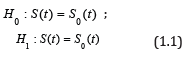
for a fixed value of t, e.g., 6 or 12 months, where S(t) = P(T > t) denotes the survival fraction and S₀(t) denotes the null survival fraction. The time-to-event variable in these trials might be overall survival or more often progression-free survival (PFS), but the exposition below does not depend on what survival endpoint is used. Traditionally, the typical phase II trial based on a survival fraction assumes that there are no censored observations prior to time t, i.e., the minimal follow-up time for a given subject is t. The specification of a minimum follow-up length t simplifies the problem to a standard binomial test, either using a single-stage exact binomial test or having the ability to employ classic two-stage or multi-stage designs as desired. We acknowledge that the assumption of no loss to follow-up prior to time t could be problematic; however, in our experience, it has not been a problem, and as discussed below, other authors [1] still recommended this approach despite this assumption. In addition, if there is some concern about loss to follow-up, the sample size could be increased slightly to account for this.

Other authors have explored issues with the use of time-to-event endpoints in single-arm phase II studies. In the two-stage design, Case et al. [2] proposed using Nelson-Aalen estimates of survival in order to prevent the need to follow all patients to time t for the interim analysis (end of stage 1), which can result in lengthy between-stage suspensions [1]. compared three approaches for this setting:

(i) Treating the endpoint as binomial (as we do here),

(ii) Using Nelson-Aalen estimates, and

(iii) A test based on the Exponential maximum likelihood estimator (MLE);

they recommended the use of the binomial endpoint given its strict control of the type I error, with the caveat that it does

require that no patients be censored before the specified time t. Other authors have proposed using a one-sample log-rank test to compare to historical controls [3]; however, this approach has the major limitation that one needs the actual data set of historical controls, rather than just summary information. While the hypothesis test at (1.1) reduces to a standard binomial test given the minimum follow-up time per subject t, the actual operating characteristics of the test depend upon both the underlying form of S(t) and the choice of t: for the null hypothesis in terms of Type I error control and for the alternative hypothesis in terms of power. To the best of our knowledge, there has been no study of the impact of the choice of t on the discreteness of the binomial test (and the resulting power ramifications), and no examination of the effect of the assumed underlying form of S(t). In addition, in these trials, the alternative hypothesis is universally framed with regard to a difference (or shift) in survival at the given time point, i.e., S1(t) = S₀(t) +δ (as is often done in a test of a binomial endpoint); however, we can, and perhaps should, at least consider framing the alternative from the typical survival perspective, i.e., S1(t)=S₀(t), where is the hazard ratio assuming proportional hazards. We illustrate in this note that under some common scenarios found in the cancer clinical trial setting, slight changes in t can lead to dramatically different values for Type I error and power; we also consider both ways of framing the alternative: proportional hazards or shift. While some of our results may appear obvious after some consideration (e.g., increasing power as t increases and thus the proportion surviving decreases), these effects have not been examined in the literature and apparently have not been considered in the design of these trials. In sections 2 and 3, we examine the type I error control and power for the single- and two-stage designs, respectively. In section 4, we discuss two examples from our experience, and in section 5, we give some recommendations for designing studies in this setting and discuss ongoing and future work.

Power and Type I Error Control: Single-Stage Design

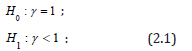
For ease of exposition we start by utilizing the assumption that the hazard function h(t) under the alternative from (1.1) is proportional to some hypothesized baseline null hazard function h₀(t), such that we have S(t)=S₀(t) under the null hypothesis and S(t)=S₀(t) under the alternative hypothesis for some hazard ratio, <1. Then we may rewrite (1.1) as

We will also examine a shift alternative under the alternative (1.1) such that we have S(t) = S₀(t) under the null hypothesis and S(t) = S₀(t) + under the alternative hypothesis for > 0. Then we may rewrite (1.1) as

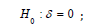
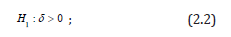
where S(t) <1: The proportional hazards alternative and the shift alternative provide different behaviors relative to the assumptions made under the alternative hypothesis. Other variations, e.g., accelerated life alternatives, would provide similar conclusions with respect to the issues below based proportional hazard or shift models and could be considered for other situations based on available information. For the purpose of illustration, we will assume a known Exponential form for the true underlying survival function under H0, given as

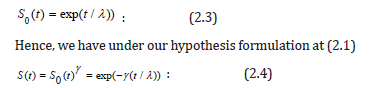
In many settings, such as a cancer cooperative group, the true underlying null distribution may be inferred fairly accurately based on historical information. The choice of the Exponential distribution is again for illustration and because of its general flexibility in terms of a general model. Other models may be more appropriate for a specific application. Similar results to what is presented below were seen (but are not shown) for Weibull models, with increasing or decreasing hazards across time. Type I Error Control. No matter what alternative we examine, e.g., proportional hazards or the shift-alternative, the Type I error behavior of the tests under consideration behaves the same since its properties are conditional on the null hypothesis. As is well-known, the actual type I error for an exact binomial test is often much less than the desired type I error due to the discreteness of the underlying test, which can make the test highly conservative [4]. However, with respect to our hypothesis (1.1), there is an opportunity to better control the true type I error rate of the exact binomial test through the choice of t such that it achieves the exact, desired -level. This simple observation alone will in turn boost the power of the corresponding fixed-level test. Minimally it will provide a better understanding regarding the ramifications of different choices for t.

An illustration, let us assume S₀(t) at (2.3) is standard exponential (λ= 5) which corresponds to a median survival time of 3.5 (and for illustration, let us say 3.5 months in terms of prescribing a unit of time). A typical test in the phase II cancer setting might be to look at the survival fraction at t =6 months, which in this case yields the hypotheses corresponding to the exact binomial test of

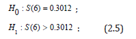
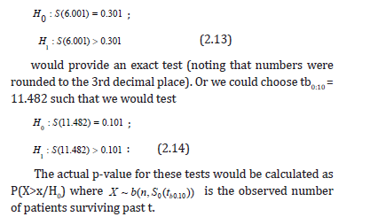
Let us examine this test at α= 0:10, n= 25 and consider other choices of t, 5.5 < t < 6.5 months. By comparison we could have chosen for example t = 6.01 such that

or a change in t of about 1/3 of a day as compared to hypothesis (2.5). Figure 1 shows the true type I error of the exact binomial test (1.1) across a range of values for t. As we can see, for very slight changes in t, the true Type I error rate, calculated from a binomial distribution, ranges from 0.0455 to 0.0990 where the minimum and maximum attainable Type I error correspond to the values for t = 6 and t = 6.01, respectively. Hence a subtle shift in t of 0.01 units has a dramatic impact on the true underlying Type I error without practically changing the hypothesis of interest, i.e., H₀: S(6) 0.3012 0 HS= compared to H₀: S(6.01) 0.3006 For a fixed sample size of n= 25 the two tests using t = 6 and t = 6:01 and a shift of S₀(t)+0.2 under the alternative yields powers of 0.6594 and 0.7896, respectively, i.e., the relative efficiency of the test at t = 6 is 84% relative to the test at t = 6:01. We would need to enroll 5 additional subjects for the test at t = 6 to have larger power as compared to the test at t = 6:01.

The saw-toothed behavior of the power curve for a one-sample binomial test has been well-characterized [4] as a function of sample size. Interestingly, in our testing framework we can achieve exact Type I error control through the choice of t. It turns out that for s sample size of n; there are n values for t corresponding to the test at (1.1) such that the desired level can be achieved precisely. The theoretical underpinnings of this process are presented next. As background notation let the incomplete beta function be denoted as

and let the regularized incomplete beta function (which is equivalent to the binomial distribution cumulative distribution function) be denoted as

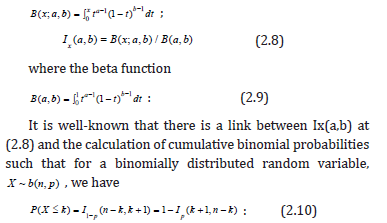
For hypothesis (1.1), we de ne b to be the upper critical value for the level test. For a sample of size n and given the one-sided direction of the test, the potential discrete values for b are 0,1,2,…,n-1, with each corresponding to a particular value of S₀(t), and thus, given an underlying form for S(t), each of these values for b correspond to a particular value of t. It turns out that there is a value of t for each b such that the desired -level is precisely the Type I error level of the test, i.e., a truly exact test. In addition, we can prove why the so called “saw-toothed” behavior occurs in this setting. Towards this end let t₀ < t₁ <…< tn_-1 denotes the n values for t such that the desired α-level is equal to the true Type I error level. This can be found by considering the regularized incomplete beta function (2.8) in the context of our test such that we solve the equation

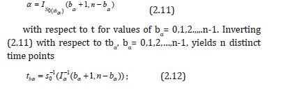
for which the test at (1.1) has precise Type I error control, where I-1 denotes the inverse regularized incomplete beta function.

An illustration, let us continue our example from above where we denote S₀(t) at (2.3) is standard exponential (λ=5) with n = 25 and = 0.10 then the n values for tb_0:10 for each b0.10 = 0,1,2,…,24 are given in Table 1. We could choose any of the values for tb_0:10 such that are our desired -level was exactly equal to the true Type I error of the test. For example we could choose tb0.10 = 6.001 such that we would test

Note. The results pertaining to the optimal choice of tb0:10 in terms of Type I error control does not depend on the form of the alternative hypothesis. In addition, the form for S₀ could be derived parametrically or using population-based data with the form of S₀ derived either semi-parametrically or nonparametrically, e.g., using kernel estimators or smoothing splines. In terms of the saw-toothed behavior seen in Figure 1, we can easily prove that IS₀(tb_α) (b_α+1, n-b_α) at (2.11) is a decreasing function to the right of any given tbα (in the interval t (tb_α,tb_α+1)) simply by taking the derivative of IS₀(t) (b_α+1,n-b_α) with respect to t and given b_α is constant in the interval t (tb_α,tb_α+1). Note that

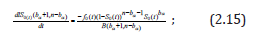
where -dS₀(t)/dt = fo(t) is the probability density function for t. Given fo(t) > 0; (1-S₀(t))n-b_α-1>0, S₀(t)b_α >0 and B(b_α+1,n-b_α)>0 proves the result.

Proportional hazards alternative: power

We know that based on the results pertaining to the Type I error provided above, the statistical power of a given test will fluctuate across values of t because the actual due Type I error rate is equal to the desired Type I error rate; we denote these as “local” fluctuations in power. There is also a “global” consideration of power across all choices of t that provide exact alpha level tests. Under our proportional hazards alternative as per (2.1) the power (1-β) is given straightforward as

1-β= IS₀(t)γ (b_α+1,n- b_α), (2.16)

where, as above, n is the sample size, b_α is the (1-β)th quantile for the binomial random variable b(n,S₀(t)), i.e., bα is the critical value of the test for a given t, and I_x(a,b) is the regularized incomplete beta function, which is defined at (2.8).

Continuing with our example S₀(t) at (2.3) being standard exponential (λ=5) with n = 25 and α=0.10, let us look at the statistical power of the test in the formulation of the hypothesis (2.1) for γ=0.6 under the alternative. The survival curves under the null and alternative assumptions are shown in Figure 2 as is the actual power as a function of t. As one can see, the same saw-toothed behavior (or “local” fluctuation) that was theoretically described above and shown in 1 for the Type I error rate is thus also seen for power across values of t (with the values for t that provide the desired Type I error level and thus maximum local power being at the values in Table 1). The global maximum power can be seen by examining the power across all of the values in Table 1. We can see the power via the choice of t can range from 0 to 0.884 at t =10.154 corresponding to one of the choices in Table 1. Practically speaking if we did what commonly occurs in practice and choose t = 6 or t = 9 months the power would be 0.659 or 0.747, respectively.

Shift alternative: power

Single-arm phase II trials are often powered to detect a specified difference, in survival at a particular time point (rather than a relative difference or hazard ratio) with the resulting alternative survival, S(t) = S₀(t)+δ, with the constraint that S₀(t)+δ≤1. The null and alternative hypotheses in this case are shown in (2.2). Figure 2 shows the null (same as in 2a) and alternative survival curves, and the resulting power under the shift alternative. As with the proportional hazards alternative, for the shift alternative, we see both the global and local pattern of fluctuating power. However, for the shift alternative, the global power is maximized when the null and alternative survival are furthest from 0.50 and is minimized when they are closest to 0.50. This contrasts to the proportional hazards alternative, under which the power is maximized when the resulting difference between S₀(t) and S1(t) is maximized.

Comment

It should be noted that under either the proportional hazards or shift alternative, the optimal t will fluctuate depending upon several design characteristics such as the underlying form of S(t) and the relative magnitude of the detectable alternative.

Power and Type I Error Control: Two Stage Design

One of the most often utilized two-stage designs in the phase II cancer clinical trials setting is due to Simon [5]. We will use the Simon two-stage optimal design, which minimizes the expected sample size under the null hypothesis, for our main points. These same ideas will translate to most other common two-stage single-arm designs about a proportion. In the two-stage setting, the saw-toothed (local) behavior demonstrated in the single-stage trial is usually a non-issue because the actual Type I error and the actual power of the test is generally close to the desired levels, α and 1-β.

However, the choice of t still has strong implications for the overall sample size due its global effects.

For the Simon design, let n₁ and n₂ denote the stage 1 and stage 2 sample sizes, respectively. The expected sample size (Simon, 1989) then is given by

ESN = n₁+ (1-PET)n₂, (3.1)

where PET=B(r₁;S(t),n₁) is the probability of early termination (i.e., at the end of stage 1), r₁ is the required number of non-failures by time t in the first stage in order to enter the second stage, and B denotes the binomial cumulative distribution function. As noted by Simon [5] the probability of rejecting the null hypothesis given success probability S(t) is

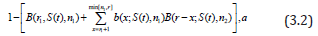
where b denotes the binomial probability density function, and r denotes the number of non-failures in both stages required in order to reject the null hypothesis. The goal is to minimize the ESN at (3.1) while constraining the value of (3.2) to be given S(t) = S₀(t) and constraining (3.2) to be ≤α given S(t)=S₀(t) under the proportional hazards assumption, or S(t)=S₀(t)+ under the shift-alternative as described above. The minimization of the ESN in this design is accomplished via a grid search, e.g., a SAS®_coded version is available [6]. The additional feature relative to our problem is consideration of the size of the study as a function of t: we could (i) minimize the ESN (which is done in the Simon optimal design) as a function of t, (ii) minimize n (which is done in the Simon minimax design) as a function of t, or (iii) minimize n₁ as a function of t. The choice of which design parameter to minimize depends our design motivations. Additionally, we could consider restricting the minimization across t to a specific range of interest, say t₁<t<t₂, e.g., restricting the range to 3 to 12 months. We examine some examples below.

Proportional hazards alternative: sample size

Let us revisit our example from the single-stage design S₀(t) at (2.3) being standard exponential (λ=5). For the Simon two-stage optimal design, we show the ESN, n₁, and n as a function of t (as integers) in Figure 3a for the alternative γ= 0.6 and with α=0.1 and β=0.1. As we can see for this particular example, there is an optimal t with respect to the global minimum ESN. Interestingly, there is a not a unique value for the minimal n₁; thus one might consider some trade offs for choice of t between a slightly higher ESN with a lower n₁, e.g., in a disease setting where active agents are rare in the historical data, there may be a desire to end a trial as soon as possible if efficacy endpoints appear unattainable. Across all the choices of the t≤20 for this example, the actual Type I error rates ranged from 0.0709 to 0.0991, and the actual Type II error rates ranged from 0.0945 to 0.1000. The optimal choice of an integer value for t in terms of the minimal ESN from Figure 3 was t =11 months. If we are interested in optimizing the design with respect to minimizing ESN, choosing t between say 7 and 12 months appears to a afford approximately equal values, and then within this range, we could select t based on minimizing n₁ or n. Obviously, choosing t closer to 0 results in dramatically larger sample sizes under our model assumptions.

In order to illustrate how the choice of t may be affected by the design parameters under the alternative, we examine the effect on the design of assuming γ= 0.5, which corresponds to a larger treatment effect than previously described with γ= 0.6. The optimal ESN as a function of the choice of integer values for t and the corresponding sample sizes are given in Figure 3b. In this case, the optimal ESN corresponds to time t=12. Across all the choices of the t≤20 for this example, the actual Type I error rates ranged from 0.0512 to 0.0995, and the actual Type II error rates ranged from 0.0896 to 0.0999.

Shift alternative: sample size

Analogous to what was seen for the examination of power for the shift alternative, we see in Figure 3c that the ESN is largest when S₀(t) and S₁(t) are closest to 0.5 (i.e., when t is close to 0.5 as shown in Figure 2). The same general pattern is seen for n₁ and n; however, there is more local variation for these than for ESN. The value of EN₀ goes to a minimum of 12.0 as t increases and as S₀(t) thus goes to zero.

Examples

As an illustration regarding the choice of t, we provide two examples. One example is from the Gynecology Oncology Group where patient-level data are available [7], and one example is the design of a trial in advanced squamous non-small-cell lung cancer, where patient-level data are not available.

Gynecology oncology group

Markman et al. [7] published a meta-analysis of seven Gynecology Oncology Croup phase II studies conducted between 1988 and 1995 to evaluate intraperitoneal (IP) therapy for partially responsive or recurrent disease. For illustration, suppose we wish to design a study around S(12), where S(12) denotes the 12 month progression free survival (PFS) rate. The actual estimated PFS curve from our 7 studies is the lower curve provided in Figure 4. In the traditional setting this would generate a set of hypotheses

with the following form:

H0: S(12) = 0.55,

H1: S(12) > 0.55, (4.1)

Suppose we wish to design a study to detect a hazard ratio, γ=0.6 at 12 months, which corresponds to S(12) = 0.70; the survival curve under this alternative (S(12|H0)γ) is the upper curve given in Figure 4. For (4.1), a single-stage design based on an exact test about a proportion at t=12, with α=0.10 and β=0.20, requires a sample size of n=49 and has actual Type I error rate of 0.095 and actual Type II error of 0.190.

For the single-stage design, the power as a function of time, given n=49 and under the proportional hazards alternative = 0.6, is shown in Figure 4. The choice of n=12 is not the optimal point within a reasonable design range of 0 < t≤20; for example, at t =19.7 months, the power is 0.92, which corresponds to the hypotheses:

H0: S(19.7) = 0.35,

H1: S(19.7) > 0.35, (4.2)

with S(19.7)= 0.53 under the alternative. Given α=0.10 and β=0.20 this would yield a sample size of n=34 as compared to n = 49 at t = 12, which may, in practical terms, actually yield similar total study times for the two designs, with t = 12 or t = 19.7). For example, if a study recruits 2 patients per month, the t=12 month design would take 24:5 months of accrual plus t=12 months of follow-up for a total of 36.5 months to complete, whereas the t=19.7 design would take 17+19.7=36.7 months to complete but would cost less due to the smaller sample size.

We could also consider a Simon optimal two-stage design for this situation: designed with t=12 months, we would require n₁ =20 (r₁=11) and n=n₁+n₂=53 (r=33), which has an actual Type I error rate of 0.0970, actual Type II error rate 0.198, and ESN = 33.7. For the two-stage design we plot n₁, n, and the ESN for t =8,…,24 with α=0.10 and β=0.20. The results are presented in Figure 4. We see that the ESN declines dramatically as a function of t, although it eventually increases (not shown) for much larger t. The other interesting feature of the plot is that, over time, there is greater variability in both the n₁ and n values than in the ESN values. As for the single-stage above, the choice of t will affect the sampln₁e size and follow-up time required, but for the two-stage design, the choice of t will also affect the first-stage sample size, which might be of particular interest. There are nontrivial differences between these competing designs such that careful consideration of the choice of t is warranted.

Squamous-cell non small-cell lung cancer

We were interested in designing a phase II clinical trial for a new agent in advanced squamous-cell non small-cell lung cancer and interested in comparing the overall survival of the new agent to a benchmark of patients receiving nivolumab. Overall survival rates at specific time points were estimated from the survival plot in the published paper of nivolumab in this disease setting and are shown as S₀(t) in Table 2 [8]. We design the trial with a shift alternative (δ=0.20) and with α=0.10 and β=0.10. The potential designs for t=3,6,9,12,15; and 18 months are shown in Table 2. Given the shift alternative, the trial is smallest when S₀(t) is furthest from 0.5, which occurs when t is small (or larger than applicable here).

Design Recommendations and Future Work

Single-arm phase II oncology clinical trials in which the primary endpoint is a time-to-event endpoint have traditionally dichotomized the endpoint around a specific time point (t) that is ostensibly chosen for some clinical or design relevance. However, to our knowledge, there has been no examination of the impact on the trial’s design and operating characteristics, including type I error rate control, power, sample size, and total trial duration (accrual plus follow-up time).

We have shown that the choice of t can have dramatic effects on the trial’s type I error control and the trial’s power (due to local effects of varying Type I error control and global effects of changing null survival probabilities, S₀(t)). A full range of values for t should be investigated to find the best choice for a given situation, where what is “best” could be affected by sample size, required trial duration (accrual and follow-up time), and of course, clinical relevance of t given the disease setting. In addition, when the endpoint of interest is progression-free survival, the timing of radiologic tumor assessments should also be considered in the choice of t; for example, scans are usually done every other cycle, and this frequency and the duration of the cycle may impact the best choice of t.

The oft-used Simon optimal two-stage design focuses on minimizing ESN, but consideration can also be given to choosing a design with a reasonable total sample size, and reasonable first-stage sample size. As Simon himself noted, if two designs have similar ESN but one has substantially smaller total sample size, then that design may be a better choice. The same consideration could be given to first-stage sample size, particularly in disease settings where even going to second stage is rare [9].

The trials discussed here are usually designed around a shift alternative (e.g.,δ=0.15 or 0.20); which is likely due to the fact that they are based on Simon-style designs. However, trialists may also want to consider the idea of the proportional hazards (or ratio) alternative when designing these trials.

Acknowledgement

“This work was supported by Roswell Park Cancer Institute and its Biostatistics Shared Resource and by National Cancer Institute (NCI) grant P30CA016056. Dr. Hutson was also supported by NCI grant P50CA159981”

BBOAJ.MS.ID.555582

Our Media Partner

BBOAJ Menu

Useful Links

Downloads

References

- Owzar K, Jung SH (2008) Designing phase II studies in cancer with time-to-event endpoints. Clin Trials 5(3): 209-221.
- Case L, Morgan T (2003) Design of phase II cancer trials evaluating survival probabilities. BMC Med Res Methodol 3(1): 6.
- Finkelstein DM, Muzikansky A, Schoenfeld DA (2003) Comparing survival of a sample to that of a standard population. J Natl Cancer Ins 95(19): 1434-1439.
- Chernick MR, Liu CY (2002) The saw-toothed behavior of power versus sample size and software solutions: Single binomial proportion using exact methods. The American Statistician 56(2): 149-155.
- Simon R (1989) Optimal two-stage designs for phase II clinical trials. Control Clin Trials 10(1): 1-10.
- Groulx A, Moon KH, Chung S (2007) Using SAS® to determine sample sizes for traditional 2-stage and adaptive 2-stage phase II cancer clinical trial designs. In SAS Global Forum. SAS 1-9.
- Markman M, Brady M, Hutson A, Berek JS (2009) Survival following second-line intraperitoneal therapy for the treatment of epithelial ovarian cancer: the gynecologic oncology group experience. Int J Gynecol Cancer 19(2): 223-229.
- Brahmer J, Reckamp KL, Baas P, Crino L, Eberhardt WE, et al. (2015) Nivolumab versus docetaxel in advanced squamous-cell non small-cell lung cancer. N Engl J Med 373(2): 123-135.
- Lachin J (1981) Introduction to sample size determination and power analysis for clinical trials. Control Clin Trials 2(2): 93-113.