


An Efficient Semiparametric Approach for Marker Gene Selection and Patient Classification
Jingjing Wu1*, Guoqiang Chen2 and Zeny Feng3
1Department of Mathematics and Statistics, University of Calgary, Canada
2Enbridge, Canada
3Department of Mathematics and Statistics, University of Guelph, Canada
Submission: December 29, 2016; Published: June 02, 2017
*Corresponding author: Jingjing Wu, Department of Mathematics and Statistics, University of Calgary, Calgary, Canada, Fax: (1-403) 282-5150, Tel: (1-403) 220-6303, Email: jinwu@ucalgaiy.ca
How to cite this article: EJingjing W, Guoqiang C , Zeny F. An Efficient Semiparametric Approach for Marker Gene Selection and Patient Classification. Biostat Biometrics Open Acc J. 2017;1(2): 555558. DOI: 10.19080/BBOAJ.2017.01.555558
Abstract
The advancement of microarray technology has greatly facilitated the research in gene expression based classification of patient samples. For example, in cancer re-search, microarray gene expression data has been used for cancer or tumor classification. When the study is only focusing on two classes, for example two different cancer types, we propose a two-sample semi parametric model to model the distributions of gene expression level for different classes. To estimate the parameters, we consider both maximum semi parametric likelihood estimate (MLE) and minimum Hellinger distance estimate (MHDE). For each gene, Wald statistic is constructed based on either the MLE or MHDE. Significance test is then performed on each gene. We exploit the idea of weighted sum of misclassification rates to develop a novel classification model, in which previously identified significant genes only are involved. To testify the usefulness of our proposed method, we consider a predictive approach. We apply our method to analyze the acute leukemia data of [1] in which a training set is used to build the classification model and the testing set is used to evaluate the accuracy of our classification model.
Keywords: Semi parametric model; Maximum semi parametric likelihood estimate; Minimum Hellinger distance estimate; Microarray data; Differentially expressed gene; Classification
Introduction
Microarray technology has made the genome-wide gene expression pro le available simultaneously. The global geneexpression analysis helps biologist and physician to better understand the path physiological mechanisms. More specifically, it helps to better understand the mechanism of a disease, such as cancer, and thus makes improvement in diagnoses and treatment strategies. Microarray gene expression based classification has been considered by [1] for acute leukemia, [2] for classification of p53-regulated genes, [3] for tumor classification, [4] for small round blue-cell tumors, [5] for large B-cell lymphoma, among others. It has been reported by [6,7] that classification using gene expression data is promising in cancer classification and, more generally, disease classification.
However, the analysis of microarray gene expression data for classification is challenging. The curse of dimensionality is a well known issue in microarray analysis. It is common that microarray data consists of expression levels of thousands of genes while only a few dozen of samples are available for analysis. This is often referred to the problem of large p (number of features, i.e., genes) and small n (sample size). When the number of genes is much larger than the number of observations, a prescreening process is often performed. In this prescreening process, significance test is performed on each gene individually to identify genes that are differentially expressed over different classes and exclude genes that are not differentially expressed for further analysis. This step helps to remove noise and reduce dimension of features for later classification analysis.
The two-sample student t test is a simple method for identifying genes that are differentially expressed over two conditions or classes. However, when sample size is small, the power of it is often low. In addition, the estimate of standard error is not stable and thus indicates the false positive error. Modified t tests have been proposed to address this issue [8]. Added a small positive constant to the denominator of the t statistic to avoid genes with small change in expression level being selected as significant. Following a similar idea [9], proposed a regularized t test for each gene by using a weighted average of gene-specific variance and global average variance in the denominator. Although the modified t statistic improves the performance of significance test over the conventional t statistic, when sample size is small, the appropriateness of using t-type tests is still questionable. Alternatively, nonparametric test, such as the Wilcoxon rank-sum test, is used to identify genes differentially expressed over different tumors in [10]. However, the Wilcoxon test is reported to be generally less powerful than the t-type tests [11]. To coordinate the pros and cons of parametric and nonparametric statistics, i.e. model flexibility and sensitivity, appropriate semi parametric methods should be considered. However, to our knowledge, least e ort so far has been given in this area. In this paper, we propose a two- sample semi parametric model for gene expression levels under different classes. We use both the classical maximum likelihood estimation (MLE) and the more robust minimum Hellinger distance estimation (MHDE) to estimate the parameters in the model. In the prescreening step, Wald statistics based on both MLE and MHDE are constructed for each gene to test whether it is differentially expressed over different classes.
The single-gene based significance test in the prescreening step helps eliminate non-differentially expressed genes from classification model. In the second step, a classification model is developed based on significant genes identified in the first step. In two class classification problems, some methods aim to learn a hyper plane to separate the two classes. This learned hyper plane can then be used to predict class membership of new incoming samples. For example, Fisher's linear discriminant analysis [3] and support vector machine (SVM) technique [1,11] are used for cancer classification. Similarity based classifiers is considered to be the most straightforward method. For example, k-nearest neighbors (k-NN) is used by [12] for cancer classification. The k-NN classifier is a nonparametric method that deter-mines a new sample's class membership based on the majority vote of class memberships of its k nearest neighbors in the training set. However, the k-NN method is very sensitive to the choice of k. When number of genes is large, the k-NN method works less efficient [6]. Other methods used in cancer or tumor classification include artificial neural networks (ANN) [4], decision tree [3] and boosting [13].
As we noted that there are few attempts have been given to semiparametric methods. Intuitively and along the same lines as in the identification of differentially expressed genes, we propose to use the same two-sample semi parametric model to estimate misclassification rates for each significant gene identified previously. With appropriately chosen weights, we employ weighted sum of misclassification rates over all significant genes to build a novel classifier.
The remainder of this paper is organized as follows. Section 2 presents the methods used in this paper for marker gene selection and patient classification. Specifically, we introduce in Subsection 2.1 the two-sample semi parametric model for gene expression levels, in Subsection 2.2, both MLE and MHDE for the parameters are constructed and discussed, Subsection 2.3 proposes a procedure for marker gene selection with use of Wald statistics based on either MLE or MHDE; and in Subsection 2.4, we develop a semi parametric classification model based on the marker genes. Section 3 presents the classification results when the proposed classification model is applied to the leukemia data in [12,13]. Particularly, Subsection 3.1 presents and compares the results of linear semi parametric model with those of quadratic semi parametric model; in Subsection 3.2, we use an altering procedure to improve the classification performance; and Subsection 3.3 discusses the robustness properties of MLE and MHDE. Finally in Section 4, we give concluding remarks and discussions.
Method
A semiparametric model
Let Y be a binary random variable that indicates the disease status of an individual. For example, in acute leukemia, we use Y=1 to denote the acute lymphoblastic leukemia (ALL) and Y =0 to denote the acute myeloid leukemia (ALL). For simplicity in description, we use the term "case" for an individual with Y=1 and \control" for an individual with Y = 0. Let X denotes the associated covariate. Here, X could represent the expression level of a gene. A logistic regression model is often used to link the covariate to the response Y as
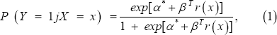
where r (x) = (r1( x),..., rp (x))T is a vector of functions of x,a is a scalar parameter, and pis a px1 vector of coefficient parameters. In most applications r (x) = x or r (x) = (x, x 2). In a retrospective study, the samples contain individuals with Y = 0 or 1 and their corresponding gene expression pro les are recorded. For a given gene, suppose the expression levels of n individuals, X1,..., Xn, is an independent and identically distributed (i.i.d.) sample from the control population with density function g( x) = f( x|Y = 0) . Independently, Xn+1,...,Xn+m is another i.i.d. sample from the case population with density function . h( x) = f( x|Y = 1) Denote Π = P(Y = 1), then (1) and Bayes's rule give the two-sample semiparametric model
Xn+1,.......Xn i.i.id. g(x)
Xn+1, , Xn+m h(x) = g(x)[α + βTr(x)], (2)
Where α is a normalizing parameter that makes g (x)[α + βT r (x)] a density. It has been shown in [14] that Models (1) and (2) are equivalent when α = α* + log[(1 -π)/ π]. The two unknown density functions g(x) and h(x) are linked by an "exponential tilt" exp[α + βrr(x)] . Let θ = (α,βT)T . Now the problem of estimating P(P(Y = 1|X = x) has been transformed to the estimation of in (2) while g is treated as a nuisance parameter.
Many inferences based on model (1] assume that the log odds,  is normally distributed. Comparatively, this semi parametric model (2] is more robust in the sense that it does not assume any specific form of the two underlying population distributions and only focuses on the relationship and difference between them. The difference in population distribution between cases and controls is respected by the parameter . When =0, the case and control population distributions are identical. In the next subsection, we propose to use both maximum semi parametric likelihood estimation (MLE) and minimum Hellinger distance estimation (MHDE) to estimate .
Parameter estimation
Maximum semi parametric likelihood estimate: Let G and H denote the cumulative distribution functions corresponding to g and h respectively. We arrange the observed data in order so that X1,...,Xn are from the control group and Xn+1 ,,...,Xn+m are from the case group. Then the likelihood function θ = (α,βT)T of under the semi parametric model (2] is given by

subject to pi ≥0 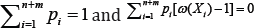 and where w(x) = exp[α + βT r(x)] and pi = dG(Xi), I =1,.., n+m. [15] has shown that the maximum value of L is attained at
where p = m / n and  the MLE of as the solution to the system of estimating equations
with 1(θ) the profile log-likelihood function given by

Note that the solution to the equation system (3) doesn’t have an analytical form, and thus a numerical method such as Newton-Raphson iteration is used for finding the solution [15].Has shown that the MLE  -consistent and asymptotically normally distributed.
Minimum hellinger distance estimate: It is generally believed that MLE is efficient in the sense of achieving the Cramer-Rao lower bound. However, it is very sensitive, and thus no robust, to model misspecification and outlying observations. On the other hand, existence of outlying observations is very common in microarray data. For instance, in the acute leukemia data analyzed by [10], there are some outlying expression levels for some genes, which can be seen from the box plots in Figure 1. When sample size is small, it is often not clear whether an outlying observation is due to measurement error or it is a true observation as it is. Simply removing outlying observations from the analysis is not appropriate as it may lead to a less powerful study. Therefore, a robust estimate against outlying observations is desired. Following this direction, we propose a minimum Hellinger distance estimate (MHDE] of the parameters in model (2).

Suppose a simple random sample is from a population with density function h, where is the only unknown parameter in a finite dimensional parameter space θ. The MHDE of θ under the parametric model is defined as

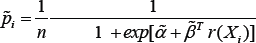
Where ĥ is an appropriate nonparametric estimator, e.g. kernel estimator, of the underlying true density based on the sample [16]. Has shown that the MHDE defined in (4) is asymptotically efficient and exhibits good robustness properties. For the two-sample semi parametric model (2),. Unfortunately, the estimate is unavailable since, besides θ , g is also unknown in hθ . Intuitively, one can use a nonparametric estimate of g based on X1,..,Xn to replace g and then get an estimated hθ. Specifically, we de ne kernel density estimates of g and hθ, respectively, as
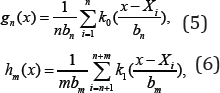
Where K0 and K1 are nonnegative kernels, bandwidths bn and bm are positive constants such that bn →0 as n! 1 b → 0 and n⟶∞ as m⟶∞ . For any , can then be estimated by
ĥθ(x) = exp[α + βTr (Xt )]gn (x). (7)
Now our proposed MHDE of and is defined as
Note that we do not impose normalization constraint ∫ĥt(x)dx=1 on t. The reason is that, even for such that is not a density, it could make a density. The true parameter value θ may not make h a density, but it is not reasonable to exclude θ as the estimate of itself. To calculate, a numerical method, such as Newton-Raphson iteration or one-step method [4] can be used. Asymptotic properties of this MHDE have been well investigated p by [17] in which this MHDE has been shown n-consistent and asymptotically normally distributed. Moreover, it is found very robust against outliers and model misspecification.
Hypothesis test for identifying differentially expressed genes
In application of finding genes that are differentially expressed over classes, we can perform hypothesis test on . For the kth gene, let gk and hk represent the density functions of expression level for control group and case group respectively.Then gk and hk follow model (2) with  . In our numerical studies in Section 3, we consider both linear form and quadratic form for in model (2), hk i.e. we take r(x) = x orr (x) = (x, x 2)T . For now we use to retain the generality of our model and method. If the kth gene is not differentially expressed over case population and control population, then θk=0. In this case, the kth gene provides no information on classification and thus should be excluded from the classification model. Note that is only a normalizing parameter depending on βk . Therefore, to test whether a gene is differentially expressed over cases and controls, we only need to test
H0 : βk = 0 v. s. H1: βk ≠ 0. (9)
Given an estimate β k of , denoted by β k*, and an estimate of its associated covariance matrix, denoted by  the Wald test statistic is given by
Here, we use forβk* either the MLE βk given by (3) or the MHDE βk given by (8). Since both estimators have been proved asymptotically normally distributed, H0 under both  and are
  distributed asymptotically.
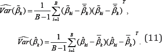
The asymptotic covariance matrices of  are given in [16] and [18,19], respectively, and therefore the covariance matrices of the two estimator can be readily estimated using the plug-in rule. However, when sample size is not large,the distribution may not approximate the exact distribution of the Wald statistic well. Due to the fact that only a few dozen of samples are available in most microarray data, we consider a nonparametric bootstrap method to estimate the covariance matrices of the estimates. In a total of B bootstrap samples, each sample is obtained by resampling subjects with replacement within each class. Each bootstrap sample has the same sample size as the original data. For the ith bootstrap sample, we compute both the MLE and MHDE, denoted by respectively.Let
 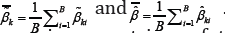 . Then the bootstrap estimates of the covariance matrices of the MLE and MHDE of are respectively given by
At a given significance level, say we compare the Wald test statistic in(10), computed with the use of either the MLE  or MHDE
 with , the 5% upper quintile of distribution. if is greater than
  , then we reject the null hypothesis that the kth gene is equally expressed over the two classes and thus include it for developing classification model in the next step.
Classification model
Suppose in the previous step s genes are identified differentially expressed over the two classes at significance level . We call these genes candidate genes. Let gk and hk denote the density functions of the kth candidate gene's expression level for control and case respectively. Given the expression level xk of the kth candidate gene of a patient, we de ne event misclassification into control at xk if this patient is in case group but misclassified into control group. We further call the probability of this event the misclassification rate into control at xk, denoted by pk0. We can similarly de ne event misclassification into case and misclassification rate into case at xk denoted by pkl. In Figure 2, we illustrate a classification scheme based on the distributions of gene expression level for the case population (hk) and control population (gk). Suppose, as shown by the top graph in Figure 2, the density curve for case (hk) is on the right side of the density curve for control (gk). For a patient with the kth candidate gene expression level xk, we classify this patient into either control group or case group. If we classify this patient as case, then reasonably any patient with the kth candidate gene expression level higher than xk will also be classified as case, and thus the yellow area under the density curve gk and on the right side of xk is pk1, the misclassification rate into case at xk.

Similarly, if we classify this patient as control, then reasonably any patient with the kth candidate gene expression level lower than xk will also be classified as control, and thus the green area under the density curve hk and on the left side of xk is pk0, the misclassification rate into control at xk. To minimize the probability of misclassification, we classify this patient into case group if pk1 < pk0, otherwise we classify this patient into control group. Reversely, if the density curve of case (hk) is on the left side, as shown by the bottom graph in Figure 2, then the yellow area under gk and on the left side of xk is pk1 and the green area under hk and on the right side of xk is pk0. Here, we call the yellow area the misclassification region into case (MCR1) at xk and the green area the misclassification region into control (MCRO) at xk.
Note that pk0 and pk1 are not available simply because gk and hk are unknown. However, we can obtain nonparametric estimators gnk and hmk of gk and hk, respectively, constructed in the same manner as in (5) and (6). By using the plug-in rule, the estimated misclassification rates into control and into case are respectively

Where Ak0 is the MCR0 and Ak1 is the MCR1 When hmk is on the right side of gnk, is the left tail probability of hmk with the right tail probability of gnk with . When hmk is on the left side of gnk, is the right tail probability of hmk with and is the left tail probability of gnk with .To decide the relative positions of gnk and hmk, one can simply compare their peak positions. Although the candidate genes identified in the previous step are all statistically significant, they are not all at the same significance level. So when we use these genes for classification, we cannot treat them equally important. Instead we give them different weights according to their significance levels to respect their different contributions to our classification model. Since the Wald statistic in (10) quantifies the significance level of the kth candidate gene, we use standardized Wald statistic
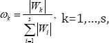
as the weight for the kth candidate gene. Now we define the overall misclassification rate (OMR) into control and that into case, respectively, as
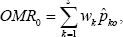
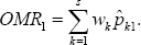
Clearly, OMR0 and OMR1 are weighted sum of misclassification rates over all candidate genes. Now our classification rule based on all s candidate genes is constructed with use of OMR0 and OMR1. We classify a patient into the case group if OMR1 < OMRO and into the control group if OMRO < OMR1. Alternately, we de ne the case classification confidence (CC) coefficient
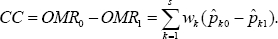
It can be shown that A CC value closer to 1 suggests a case patient and a CC value closer to -1 suggests a control patient. We summarize our classification rule as
Classified as a case if CC > 0,
Undeterminedif CC = 0, (12)
Classified as a control if CC < 0:
By now we have developed a two-step procedure for gene- based classification problem. In the first step, we perform significance test to identify genes that are differentially expressed over different classes. In the second step, we classify patient samples to either case group or control group using the expression pro le of these candidate genes. This two-step procedure is natural, consistent and self-contained in the sense that the same semi parametric model (2) is utilized in both steps and the methodologies used in the two steps are closely connected and one doesn't need to combine two different scenarios for significant gene selection and patient classification.
For the simplest case of model (2), we let and thus h( x) = g (x)exp[α + β1x] . To simplify referencing, we refer to this model as the linear semi parametric model. In many situations, linear semi parametric model would not be able to model the difference in distribution variance between case group and control group. For example, if the expression level of a gene in the control group follows a N(0,1) distribution and that in the case group follows a N(μ,σ2) distribution, then  and α = -logσ-μ2/(2σ2), with α = - logσ-μ2/(2σ2), and h(x) = exp[α + β1x+β2x2]g(x). β2 = 1/2-1/(2σ2) Note that β2= 0 is equivalent to σ2 = 1 , i.e. the two distributions have the same variance. This indicates that an additional quadratic term in the semi parametric model (2) would help to model the difference in distribution variance between case population and control population. Here, we refer to the model including both linear term and quadratic term as the quadratic semi parametric model. In other words, the quadratic semi parametric model takes r( x) = (x, x2)T . We apply both the linear and the quadratic semi parametric models to our numerical studies in the next section.
Application to leukemia study
Classification using proposed methods
In this section, we apply our proposed classification model to a real acute leukemia data. This acute leukemia data was first analyzed by [12] and it contains gene expression levels of two types of acute leukemia patients: acute lymphoblastic leukemia (ALL) and acute myeloid leukemia (AML). This data set consists of 27 ALL and 11 AML patients. For each patient, a bone marrow sample was collected and a microarray gene expression pro le for 6817 human genes was produced by an ymetrix. We refer to this data set as the training set to which our two-step procedure will be applied to build the classification model. The performance of the so built model will be evaluated through an independent testing set which contains 34 acute leukemia patients with 20 ALL and 14 AML samples. In the first step of the procedure, to calculate the MHDE of k for the kth gene, one needs to choose appropriate kernels and bandwidths for nonparametric estimates gn and hm given in (5) and (6) respectively. Here we use the following truncated standard normal kernel for both K0 in (5) and K1 in (6):
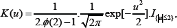
Where I{|u|≤2} is the indicator function that takes value one when and otherwise zero, and is the cumulative distribution function of N (0,1). For the bandwidths in the two kernels, we choose adaptive bandwidths
bn = Snhn and bm = Smhm ,
Where Sm = 1 1926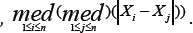 , Sm = 1.1926 .
 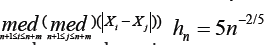 and hm = 5m-2/5.Here Sn and Sm the robust scale estimators proposed by [17]. The rational of choosing constant 5 in and is given in (6). This choice of bandwidths satisfies the conditions on bandwidths that are required to obtain the asymptotic normality of the MHDE given in (8) [20]. Under the linear semi parametric model, to estimate the variances of the MLE and the MHDE by using (11), we generate B = 50 bootstrap samples. At 5% significance level, we test the hypotheses in (9). Using Wald test statistics based on the MLE 'S, there are 620 genes differentially expressed over the ALL group and the AML group. Using the MHDE 'S, there are 653 genes differentially expressed over the two groups. In the second step, we t classification models using these two different set of candidate genes. When applying the two classification models to the training set, two patients among the 38 are misclassified regardless of which set of candidate genes is used. When using the two models to classify patients in the independent testing set, three patients among the 34 are misclassified regardless of which model is used. From these results, we see that both MLE and MHDE are very competitive with the same misclassification rates for this leukemia data. Under the quadratic semi parametric model and still at 5% significance level, a set of either 89 or 26 candidate genes are found to be differentially expressed over the ALL group and the AML group when using either the MLE or the MHDE correspondingly In comparison with the linear semi parametric model, much fewer genes are found significant when the quadratic term is added. Under the quadratic semi parametric model, the subsequent classification model, involving either set of candidate genes, classifies all patients in the training set correctly. However, when the two classification models are used to classify the patients in the testing set, five patients are misclassified by the classification model with use of the MLE and six patients are misclassified by the classification model with use of the MHDE.

In the comparison between the linear semi parametric model and the quadratic semi-parametric model, the quadratic semi parametric model is more complex. When the two underlying distributions g and h in model (2) have difference in variance, the quadratic semi parametric model may help to model them better. Figure 3 uses the 28th gene in the training data to illustrate the improvement in density estimate when the quadratic semi parametric model is used over the linear semi parametric model. For all the graphs in Figure 3, the yellow and green solid lines represent the nonparametric kernel density estimates gn and hm respectively. In the top two graphs, the dashed green line represents the estimate of the density function for the AML group using the MLE (left graph) and MHDE (right graph) under the linear semi parametric model, i.e. the estimated semi parametric model (7) with and replaced by either (left graph) or (right graph). The dashed green lines in the two bottom graphs represent the estimate using the MLE (left graph) and MHDE (right graph) under the quadratic semi parametric model. It can been seen that, when the distributions of gene expression for the two groups have different variances, the density estimate for the AML group under the quadratic semi parametric model is much closer to the nonparametric density estimate than the estimate under the linear semi parametric model, regardless of either MLE or MHDE is used. Thus, the quadratic semi parametric model helps distinguish the difference in distribution between the ALL group and the AML group better. Similar phenomenon is observed for some other genes.
Filtering candidate genes
We have shown that having the quadratic term in the semi parametric model may help to t the model better in some situations. However, this model is more complex and sometimes may over t data when sample size is small. This is respected by the lower accuracy rate when the classification rule based on the quadratic semi parametric model is applied to the testing leukemia set. Thus, when sample size is small, a simpler model is preferred to avoid over fitting problem. On the other hand, when the linear semi parametric model is used, there are too many candidate genes included for the development of classification models. In our two-step procedure, the first screening step is used to exclude genes that are not informative from classification models. However, there are still 620 significant genes with use of the MLE and 653 significant genes with use of the MHDE. Many of the false significant genes arise due to the correlations with some true marker genes. Therefore, we consider in the following an additional filtering step to further remove some irrelevant genes from the classification model.
Based on the kth significant gene identified in the first step, we classify each patient in the training set by comparing the misclassification rate into ALL, pk0, and that into AML, pkl, as described in Subsection 2.4. Then we can calculate the accuracy rate of classification based on the kth significant gene over all patients in the training set. After calculating classification accuracy rates for all significant genes, we remove those significant genes with lower accuracy rates and keep those with higher accuracy rates. To keep our classification model simple, we choose a high classification rate of 80% as a threshold. With this threshold, we have only 22 genes left when using MLE and 31 genes left when using MHDE. Now we fit new classification models based on these two filtered gene sets. When the classification models based the filtered gene sets are used to classify patients in the training set, the classification model with use of the MLE misclassifies one patient and the model with use of the MHDE classifies all patients correctly. When the classification models with filtered gene sets are applied to the independent testing set, the model with use of MLE misclassifies one patient and the model with use of MHDE misclassifies four patients.
We compare our classification results with those in [12]. Used a class predictor by comparing weighted vote for ALL and that for AML, based on a set of 50 prescreened genes. They used prediction strength of 0.3 as a threshold so that whenever prediction strength is lower than 0.3 they would say that the classification of this patient is uncertain. To be comparable, we remove this threshold to classify all patients. As a result, they misclassified one patient in the training set and two patients in the independent set. Therefore, our classification model with altering based on MLE performs better than the weighted vote class predictor in [12]. Also note that our classification model with altering based on MLE only involves 22 marker genes while that of [12] used 50 genes.
Comparison between MLE and MHDE
In this section, we compare the robustness properties of the MLE and the MHDE through the analysis of the leukemia data. Specifically, we examine the behavior of the MLE and the MHDE when outlying values are present. For simplicity, we only look at the case when the sample is contaminated by a single outlying value. Cases of more than one outlying value give similar results.
To study the robustness, we look at the change in the estimate, either the MLE or the MHDE, before and after data contamination. If the change is small, then it indicates that the estimate is not sensitive to outlying observations and thus robust; otherwise the estimate is not robust to outlying observations. To deliberately contaminate the training data, we replace the median expression level of the kth gene of all AML patients with an outlying value z. To see how the position of the outlying values affects the estimate, we allow the outlying values vary. Specifically, we take total 3501 different z values
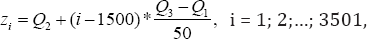
Where Qi is the ith quartile of the kth gene expression level of all AML patients. Note that both ALL group and AML group could be contaminated by outlying observations. We only consider the case that the AML group is contaminated, and similar results apply to the other case as well. To measure the change in the estimate before and after data contamination, one can use the -influence function of the estimate given by [15]. Here we use an adapted version of the applied by [20,21], and among many others. Since the training set includes 38 patients,the contamination rate is then 1/38 and the (α - IF) is given by
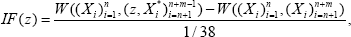
Where W represents any estimator of based on the data from both g and h, and(z,X*n+1,...,x*n+m_1) is the contaminated data with the median (X n+1,..., Xn+m ) of replaced by an outlying value z. In our study, W is either MLE or MHDE . We don't bother to give the (α- if ) of estimates of (normalizing parameter) due to the fact that it is a function of . We calculate the (α- if ) for each single gene and results for some randomly selected genes are presented in Figure 4. Similar graphs are observed for other genes.

The most striking observation of Figure 4 is that, the (α- IF) of the MLE fluctuates a lot while that of the MHDE is very stable when the outlying value z varies. As the outlying value z increases in its absolute value, the (α- if of the MHDE appears to converge to a Constant. In fact, the absolute value of the (α- if of reaches its peaks when z is around median and then slides down to zero baseline on both directions. For the MLE , however, its (α- IF) increases dramatically when the outlying value z moves to right from median. When z is smaller than median, and
  are competitive with (α - IF) s very close to each other but still has larger (α-IF) in absolute value than for most genes in Figure 4. Jumps in seems to occur possibly everywhere and are relatively big sometimes. Comparatively, it seems that jumps in only occur when z is far away on the right side of median but with high frequency. We believe that these small jumps in b are due to the control of number of iterations when doing optimization since they all look uniform. All these observations support our conclusion that the MHDE is much more robust than the MLE against outlying observations.
The very different behavior of on left side and right side of median could be expected from the fact that the semiparametric likelihood is proportional in some sense to the quantity Without an outlying value, is a negative value no matter which gene in Figure 4 we look at. When the outlying value z is negative with large absolute value,
 is not an extremely small value and therefore is not much affected. If z is a positive large value, then
 will be extremely small and the maximizing process will tend to assign a positive value, and as a result the (α-IF) will be positive and relatively large as shown in Figure 4.
When data is contaminated by outlying observations, the MLE will be affected and change a lot. As a result, after contamination, originally significant genes identified by MLE may not be significant anymore and other non significant genes may be identified by MLE as significant as well. In other words, if the data is contaminated, then one will probably pick up wrong significant genes and then make unreliable classification of patients. Comparatively, the MHDE will most likely give very consistent significant gene selection and patient classification even when data is contaminated. Therefore, even though the MHDE may not be as e cient as the MLE, the MHDE is also a good choice since it is much more robust than MLE, and these two methods should carry each other.
Discussion
In this article, a two-sample semi parametric model is proposed to model how a binary disease status is related to gene expression levels. Based on both the MLE and the MHDE, a natural, consistent and self-contained classification model is proposed and tested on a leukemia data. With simple altering, the classification model based on MLE outperforms the weighted vote predictor in [12]. In general the classification models based on MLE and MHDE are quite competitive in the sense of efficiency and robustness and both are very promising in marker gene selection and patient classification. Although we considered adding quadratic term and altering marker genes to improve the performance of classification model, there still is noise contained in the classification model. To remove the noise and get a more reliable classification model, an intuitive way is to look at directly the chance of being in control group or case group based on each single significant gene. Since we have the estimation of parameters in model (2), one can easily estimate the parameters in model (1) according to the relationships between the two models. Then one can get estimation of the chance of being a control or a case by (1). With appropriate weights, one can use the weighted sum of chances of being a control over all significant genes and that of being a case to build a classification rule. Second, one could test the hypothesis on the quadratic term coefficient β2(i.e.H0: β2 = 0v.s.Hl: β2 ≠ 0) to decide which r(x), either r(x) = x or r(x) = (x, x2)T, is more appropriate for each single gene. Third, double-weight could be used. For example, one could multiply the original weight by another penalty weight that is proportional to the maximized log-likelihood or the reciprocal of the minimized Hellinger distance.
Acknowledgement
The authors acknowledge with gratitude the support for this research via Discovery Grants from National Science and Engineering Council (NSERC) of Canada.
References
- Golub TR, Slonim DK, Tamayo P, Huard C, Gaasenbeek M, et al. (1999) Molecular classi cation of cancer: class discovery and class prediction by gene expression monitoring. Science 286(5439): 531-537.
- Yu J, Zhang L, Huang PM, Rago C, Kinzler KW, et al. (1999) Identification and classification of p53-regulated genes. Proc Natl Acad Sci U S A 96(25): 14517-14522.
- Furey T, Cristianini N, Duffy N, Bednarski D, Schummer M, et al. (2001) Support vector machine classification and validation of cancer tissue samples using microarray expression data. Bioinformatics 16(10): 906-914.
- Khan J, Wei JS, Ringner M, Saal LH, Ladanyi M, et al. (2001) Classification and diagnostic prediction of cancers using gene expression pro ling and artificial neural networks. Nature Medicine 7(6): 673-679.
- Alizadeh AA, Eisen MB, Davis RE, Ma C, Lossos IS, et al. (2000) Distinct types of diffuse large B-cell lymphoma identified by gene expression pro ling. Nature 403(6769): 503-511.
- Lu Y, Han J (2003) Cancer classification using gene expression data. Information System - Special issue: Data management in bioinformatics 28(4): 243-268.
- Asyali M, Colak D, Demirkaya O, Inan MS (2006) Gene Expression Profile Classification: A Review. Current Bioinformatics 1(1): 55-73.
- /a> Tusher VG, Tibshirani R, Chu G (2001) Significance analysi s of microarrays applied to the ionizing radiation response. Proc Natl Acad Sci 98(9): 5116-5121.
- Baldi P, Long AD (2001) A Bayesian framework for the analysis of microarray expression data: regularized t-test and statistical inferences of gene changes. Bioinformatics 17(6): 509-519.
- Tschentscher F, Husing J, Holter T, Kruse E, Dresen IG, (2003) Tumor classification based on gene expression profiling shows that uveal melanomas with and without monosomy 3 represent two distinct entities. Can Res 63(10): 2578-2584.
- Karunamuni RJ, Wu J (2011) One-step minimum Hellinger distance estimation. Computational Statistics and Data Analysis 55: 3148-3164.
- Ben-Dor A, Bruhn L, Friedman N, Nachman I, Schummer M, et al. (2000) Tissue classification with gene expression profiles. Journal of Computational Biology 7(3-4): 559-583.
- Jeanmougin M, de Reynies A, Marisa L, Paccard C, Nuel G, et al. (2010) Should we abandon the t-test in the analysis of gene expression microarray Data: a comparison of variance modeling strategies. PLoS ONE 5(9): e12336.
- Qin J, Zhang B (1997) A goodness of fit test for logistic regression models based on case-control data. Biometrika 84(3): 609-618.
- Dettling M, Buhlmann P (2003) Boosting for tumor classification with gene expression data. Bioinformatics 19(9): 1061-1069.
- Zhang B (2000) Quantile estimation under a two-sample semi- parametric model. Bernoulli 6(3): 491-511.
- Beran R (1977) Minimum Hellinger distance estimators for parametric models. The Annals of Statistics 5(3): 445-463.
- Wu J, Karunamuni RJ, Zhang B (2010) Minimum Hellinger distance estimation in a two-sample semiparametric model. Journal of Multivariate Analysis 101: 1102-1122.
- Rousseeuw PJ, Croux C (1993) Alternatives to the median absolute deviation. Journal of the American Statistical Association 88: 12731283.
- Chen G (2012) A Semiparametric Model for Marker Gene Selection and Acute Leukemia Classification. M.Sc. thesis, University of Calgary, Canada, pp. 1-94.
- Lu Z, Hui YV, Lee AH (2003) Minimum Hellinger distance estimation for finite mixtures of Poisson regression models and its applications. Biometrics 59: 1016-1026.


