


Abstract
The arbitrary moving charges as well as the electric currents interactions (magnetic field) are described according to the “Huygens principle model”. The magnetic phenomena interpretation rests actual despite the long story. This research completes the discussion began in the previous two articles [1,2] and based on the “Huygens principle model” application to the electromagnetic phenomena on the whole. The expressions of the strengths (force and counterforce) according to this model are evaluated as well as simplest magnetic strengths (straight conductor’s currents, wind current and solenoid) according to this model. The interactions between these conductor’s currents and arbitrary moving free charge are calculated and compared with the classical results.
Keywords:Huygens Principle; Magnetic Strength; Lorentz and Biot-Savart Laws; Ampère Force
Introduction
In [2] the interaction force between arbitrary moving charges has been calculated according to the Huygens principle, not according to the classical approach. It has been done just because there are many paradoxes concerning a magnetic field noted, for instance, in [3,4]. There are around 9 different magnetic force expressions (the Lorentz, Ampère, Weber among them) as well as there are different ether (aether) models implying such variety of expressions [2]. Besides many general (conceptual) arguments given in [2] in favor of the Huygens principle model instead of the classical (Maxwell’s electrodynamics) description there is another important one. It is the replacement of the “field description” introduced by Lagrange to abolish the Newton’s “interaction through empty space” (though Newton himself has never considered such an idea) in favor to continuous transmission of any interaction. This replacement is based on the purely geometrical approach really used by Newton. However, the arbitrary moving charges interaction formulas deduced in [4] are not strictly based on this principle just because differential operators such as grad, div, rot were used in the evaluation. Thus, the goal to evaluate the “magnetic strength” from simple cinematic ideas without the “magnetic field introduction” has not been achieved.
In [2] and previously [3] has been emphasized that: “… Maxwell’s equations (ME) are nothing but the charges at rest fields’ transformation formulae under the Galileo Transformations …it means that ME are somehow excessive – only two former equations are sufficient, that is the magnetic field H plays the subsidiary role”. Thus, this field is somehow useless in the case of arbitrary moving free charges, not the electroneutral currents’ conductors. Besides, the SR (Special Relativity) principle used in the evaluation in [4] denies the dependence of the spherical front speed relative to the “probe charge” upon its speed. So, the auxiliary factor accounting this dependence may be introduced. At last, only the 1D motion (along the line connecting charges) has been considered in detail. So, the generalization on the 3D case is needed. To finish the systematic Huygens principle model description, we are to calculate some dependences and show their plots for the current element acting on the probe charge q moving with the arbitrary “reduced” (to the speed of light) speed β1 (as it has been promised in the end of [2]). But first of all, we are to revise the expressions describing the interaction between the active charge moving with the speed β2 and the probe one moving with β1. It must be noted that charges are not the elementary ones (electron or proton) but the physically small ones, say little charged water drops, that is containing rather large quantity of elementary charges. To evaluate the elementary charges interaction law, the Huygens model is quite insufficient.
The arbitrary moving charges interaction
The main basic assumptions of the Huygens principle model are:
The existence of the “absolute space” (laboratory frame)
The strength acting from the 2nd (acting) charge onto the 1st (probe) one is inversely proportional to the distance square between them (spherical front) but not in the “moment of interaction” that is in the moment of the front arrival but in the moment of this front emission (active charge) and this front hitting at the probe charge. There is no difference between the interaction of the same and opposite sign charges (attraction) moving with arbitrary speeds, though it is not evident in contrast to the repulsion (the Ritz “ballistic model” [5]). Denoting the vector connecting the charges in the interaction moment as R = nR and the vector connecting the emission and arrival points as R’ = n’ R’ (n and n’ are the unit vectors) and recalling that the force acts also along the R’ direction (normal to the spherical front surface) one can immediately write the modified Coulomb’s law accounting the charges mutual movement:

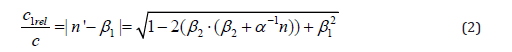
where c1rel/c is the front’s reduced speed relative to the probe charge. (This auxiliary term may be excessive and is introduced simply to describe somehow the momentum conservation law. The formulas without this term given in [2] describe only the nonlocality and time delay).
Thus, we are to rewrite some of the [2] formulas. The unit vector of the “dashed” value R’ is equal to:
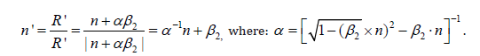
So,|R'|=αR . It’s easily shown that the ratio c1rel/c is equal to the difference module:
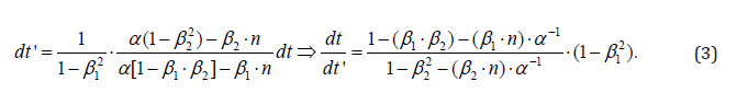
Thus, to finish with the evaluation one has simply to calculate the ratio dt/dt'. It may be done from the obvious relation:

So, one gets the quadratic equation for dt’ which solution may be expanded in Maclaurin series with the accuracy of linear terms. Finally, one gets:
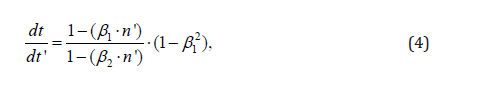
Replacing n by n’ one gets
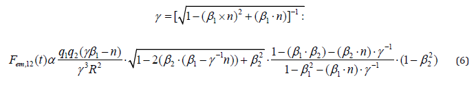
That is equal to the tangential Doppler effect (neglecting the β12 term): the strength decreases with the probe charge’s speed aligned on n’ (the probe charge runs away from the active one) and increases with active charge’s speed aligned on n’ (the active charge overtakes the probe one). Finally, the full “electromagnetic strength” expression (in the moment of interaction t) according to the Huygens principle model looks like (the subscript “21” means the active charge “2” and the probe one “1”):
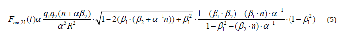
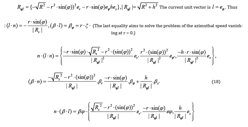
It’s evident that the 3rd Newton law does not take place. Rewriting relations (1 – 5) one gets denoting
The counterforce is not only directed along (−n +γβ1), but its module is not equal to the “force module”.
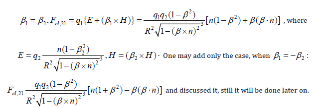
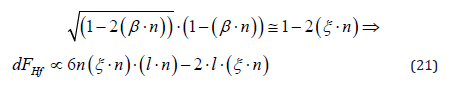
It’s easily seen that Fem,21(t) = -Fem12(t) (the 3rd Newton law is true) only when β1=−β2 just because in this case charges move symmetrically relative to each other in the absolute (ether) frame. Never mind whether they run away from each other along the same straight line or rotate (in the moment t) around the center of the intercept connecting them (like the water flowing away from the Segner wheel) the force is modulo equal to the counterforce. Decomposing the expression (5) onto the components directed along n and normal to it on gets the “electric” and “magnetic” components (that is along and normal to n):
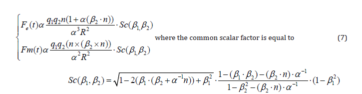
It’s easily seen that their dependence upon charges’ speeds is far more complex than the classical one though clearly interpreted according to the (1) evolution. The proportionality sign “ ∝ ” is used instead of equality simply due to the lack of sufficient proofs (yet) and independence of the units system. To illustrate this dependence let’s show some plots calculated according to (5) for equal unit charges (q1=q2) and unit distance (R=1). It is useless to compare the classical and “Huygens principle” strengths just because the classical ones are thoroughly discussed in [4] for the case of equal charges speeds:
It’s more interesting to compare accelerations calculated according to the Huygens model and the “relativistic one” that is accounting the pulse’s dependence on c (see, for instance, [6, p.74]):

When β1=β2= β this acceleration has no component normal to n and is proportional to
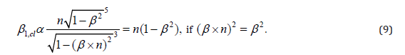
In the opposite case −β1=β2= β this acceleration is proportional to

Decomposing (as above) β = n(β ⋅n) + (n×(β × n)) on gets the “electric” and “magnetic” accelerations:

It’s quite important that the classical “magnetic” acceleration exists only when both speeds’ components exist whereas the “electric” one always exists. Still, it is rather small, negative and practically constant.
On the other hand, the Huygens model in the same case β1=-β2= β gives

(the subscript “f” – full means the full expression containing crel/c).
It’s easily seen that this acceleration does depend upon the relative charges’ motion and has normal to n component. When (β ⋅ n) < 0,(β × n) = 0 − the charges run away from each other the acceleration is less than the acceleration in the opposite case when they approach each other. However, the acceleration without this term:
 does not depend upon this relative motion as well as the
classical one. On the figure 1 the comparison of the Huygens model’s and the “relativistic one” accelerations of the probe
charge along n, that is “electric”, is presented for two different relative motions and equal speeds modules β .
does not depend upon this relative motion as well as the
classical one. On the figure 1 the comparison of the Huygens model’s and the “relativistic one” accelerations of the probe
charge along n, that is “electric”, is presented for two different relative motions and equal speeds modules β .

As it’s seen the classical “electric” acceleration falls down a little bit quicker with speed than the Huygens one regardless of the relative charges motion (not the full model!). But the full Huygens model gives quite different dependencies for approaching and running away charges. The speeds range is specially taken from 0 to 0.4c (though unattainable for water drops and even hardly achieved for heavy metals’ ions as “physically small charges”) just to show the gentle maximum reached around 0.2c. As for the running away charges the full Huygens model gives practically straight downing line. Thus, we have got some “commonsense reason” in favor of the Huygens model, still, quite insufficient to make the definite choice. Now let’s compare the normal or “magnetic” accelerations calculated according to the Huygens model and its “full version”. It is enough to consider 3 “mostly pronounced” variants: the probes move normal to n and opposite to each other, normal to each other and parallel to each other (the case discussed in [4]). The classical normal acceleration, as mentioned above, is negative, practically constant and small.
It’s seen that the “full Huygens model” normal or “magnetic” accelerations look less expressive. Therefore, accounting both figures the “full model” seems preferable. It means that the formulas (18-20) given in [2] may be rewritten according to (5-7). Though, the “conservative viewpoint” implies the auxiliary term excessive.
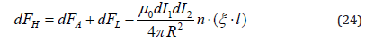
The finite length straight current interaction with a probe charge
The classical description of the straight current element and a probe charge gives only the magnetic or Lorentz force
(this term will be used in the case of currents interaction instead of “the Ampère force with the magnetic induction according
to the Biot-Savart law”): dFL = q(v× dB) where  Thus, the Lorentz force
element is equal in SI to:
Thus, the Lorentz force
element is equal in SI to:

To evaluate the proper expression of the “current – charge” force according to the Huygens model described in the
previous section (not the “full one” – conservative viewpoint) we are to express the charge’s elements corresponding
to the linear current element. (Of course, the total charge is zero – the conductor is electroneutral.) The “active positive
charge linear density” is as usually lin w . Whereas, the “active negative charge’s linear density” expressed in terms of an electric current linear density j is the ratio of this current element dI = ljd = L = ldI (l – the unit vector)
and the averaged current electrons speed
. Whereas, the “active negative charge’s linear density” expressed in terms of an electric current linear density j is the ratio of this current element dI = ljd = L = ldI (l – the unit vector)
and the averaged current electrons speed  . It is well-known that this speed is quite small (see [2]) but can slightly vary with the applied voltage. That is why one cannot truly calculate the force but can appreciate it with sufficient
accuracy. Thus, we are to rewrite the interaction formula (5+7) for the force element simply using the factor
. It is well-known that this speed is quite small (see [2]) but can slightly vary with the applied voltage. That is why one cannot truly calculate the force but can appreciate it with sufficient
accuracy. Thus, we are to rewrite the interaction formula (5+7) for the force element simply using the factor
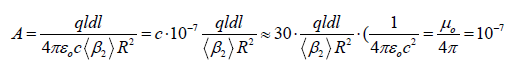 According to the 0 ε definition in the SI
system), where dI – is the current element, q – the probe charge (omitting for short the subscript “1”). As usually to calculate
the averaged speed one has to know its distribution. Fortunately, one needn’t do it just because of its smallness.
Expanding the rewritten expression in Maclaurin series with the accuracy of
According to the 0 ε definition in the SI
system), where dI – is the current element, q – the probe charge (omitting for short the subscript “1”). As usually to calculate
the averaged speed one has to know its distribution. Fortunately, one needn’t do it just because of its smallness.
Expanding the rewritten expression in Maclaurin series with the accuracy of  (linear terms) one gets the “annihilation” of the “zero” expansion term and the immobile positive charges contribution term as well as the contraction
of the same factors proportional to β2 in the nominator and denominator. The next step is the derivative evaluation.
Denoting for short
(linear terms) one gets the “annihilation” of the “zero” expansion term and the immobile positive charges contribution term as well as the contraction
of the same factors proportional to β2 in the nominator and denominator. The next step is the derivative evaluation.
Denoting for short  one gets:

Where (the term (1−β2) is omitted due to its smallness):

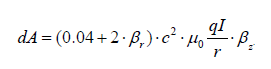
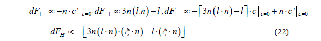
After summing contributions according to (14) of immobile positive and moving negative current’s charges one gets the Huygens force element:

(The term l(l ⋅ n) becomes zero after integration along the infinite wire.) In the cylindrical frame, l =ez the current element is {0,0, z}and the initially immobile charge point is r0={r,0,0} Thus:

After integration along the infinite wire one gets the final result:
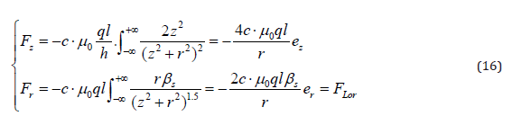
This auxiliary force Fz leads to the current decrease by the probe charge(s) motion due to the counterforce in full accordance with the principle of conservation of energy. The axial acceleration vanishes when the radial speed produced by the Lorentz force becomes βr= -0.02. Still, it is hardly possible (or even impossible) to express this auxiliary force as the potential one, that is Fz(r)= −∇ψaux(r )to write this law explicitly just because this force depends upon ez=k not upon n. That is why it is hardly possible to write the Lagrange function or canonical equations according to the Huygens model as mentioned in [1,2] (regardless the used model). As for the “magnetic field work”, it certainly exists, at least for the interaction of an infinite current and a free charge:
The solution of the motion equations system according to (16) – the ODE (Ordinary Differential Equation) system is rather simple in the case of the probe charge’s initial azimuthal speed absence. The motion is flat that is lies in the plane φ = Const. But if it is not zero the (16) system ceases to be autonomous that is depends explicitly upon time. To solve it one may certainly write (according to the azimuthal force absence):

Thus, in the rhs (right hand side) of the 2nd second equation of (16) occurs another auxiliary force m..r(t).After system solution one may calculate the ϕ (t) as the quadrature of the equation. . Thus the complete solution is obtained. The plots of the corresponding trajectories will be shown elsewhere. Now let’s estimate the real value of
the auxiliary force. Of course, the “unit charge” is too large to be considered. One may imagine some experiment like the
well-known Milliken one. Let in the vacuum chamber water drops of, say, 10μm radius, freely fall down with the gravity
acceleration ~10m/s2. Their capacity is around 10-15F and mass is around 4*10-12kg. Being charged somehow, say by the
ultraviolet emission, to the potential of 100V they obtain the charge of around 10-13C. Thus, to stop their falling down it
is enough to switch on the permanent current of around 100A. If one adds the permanent electric field (up to 1kV/m) by
means of the adjustable capacitor just like in the original experiment and the microscope to watch the process one may
come to the unambiguous conclusion about the Huygens model justice. Let us now show the analogous dependencies for
the “full Huygens model” in comparison with the classical Lorentz force – figure 3.
. Thus the complete solution is obtained. The plots of the corresponding trajectories will be shown elsewhere. Now let’s estimate the real value of
the auxiliary force. Of course, the “unit charge” is too large to be considered. One may imagine some experiment like the
well-known Milliken one. Let in the vacuum chamber water drops of, say, 10μm radius, freely fall down with the gravity
acceleration ~10m/s2. Their capacity is around 10-15F and mass is around 4*10-12kg. Being charged somehow, say by the
ultraviolet emission, to the potential of 100V they obtain the charge of around 10-13C. Thus, to stop their falling down it
is enough to switch on the permanent current of around 100A. If one adds the permanent electric field (up to 1kV/m) by
means of the adjustable capacitor just like in the original experiment and the microscope to watch the process one may
come to the unambiguous conclusion about the Huygens model justice. Let us now show the analogous dependencies for
the “full Huygens model” in comparison with the classical Lorentz force – figure 3.

Instead of the coincidence of the “Huygens model” normal force with the classical one, the “full Huygens model” gives the force of the opposite sign and approximately 1.5 times weaker in module depend less the speed and distance. It is quite remarkable just because for charges both models give the same sign (figure 2). On the other hand, this full model gives zero tangential force at the zero-probe charge’s speed. Thus, according to the full model “the magnetic field” does not act on the immobile probe charge. Never mind, which model is right and why, the main experimental fact is the attraction of the parallel currents of the same sign (see later).

The wind current and solenoid interaction with a probe charge
As one might expect using the previous section results the initially immobile free charge lying in the wind plane will be azimuthally accelerated due to the auxiliary force and then shifted in its center due to the Lorentz one and finally tending to the stable focus or stopped due to some kind of friction. Besides, the position in the wind plane is quite unstable, so the charge will be repulsed up or down this plane. As for the solenoid interaction with a probe charge, it is much more complex and strongly depends upon the sign and initial position.
Let’s begin with the wind with current I of radius R lying in the plane XY normal to the axis Z. Its element in the cylindrical frame is {R, Rϕ,0} Whereas the probe charge initial position is {p,0, h}. Thus the distance between the charge and the current element is (Cartesian frame):
Integration around the wind according to (15) leads to the constant “negative” acceleration along the current (azimuthal) as well as for the straight current (clockwise if the current flows counter-clockwise). It depends almost hyperbolically upon the distance between the charge and wind as well as upon the axial distance. As for the radial and axial forces, they are practically equal to the Lorentz ones as it was expected – see Figure 4. The Lorentz forces are obviously calculated ac-cording to the formulas:


(The Lorentz force is taken negative in the Figure 4 to account the negative probe charge just to compare with the Huygens forces). These axial forces are strongly nonlinear and changes their signs in the wind plane. It provides the attraction of the “same directed” probe charge currents like the permanent magnets. The wind’s “North pole” attracts the rotating probe charge’s “South pole” and vice versa. Due to the negative sign of the azimuthal speed the probe charge initially located in the wind plane will be shifted in its center and finally tending to the stable focus or stopped due to some kind of friction. The charges trajectories are Archimedes spirals – clockwise for positive charges (looking in the negative Z axis direction) and counter-clock-wise for negative regardless their position relative to the wind plane – above or below. These trajectories degrade into the circumferences at the initial probe charge distance from the Z axis r→0. The interaction between separate winds themselves will be considered later.
To finish with this case, it’s worthwhile to emphasis the principle difference between straight and wind currents’ interaction with a probe charge. If the straight current tries to stick it, though generating the counter force depending upon its speed, the wind current at the contrary repulses it to the axis. However, both behaviors are the energy conservation law consequences. Now let’s consider the solenoid case. First of all, it is worthwhile to note that its “theory” is much more complex and interesting. Suffice it to say that almost in every electrodynamics course only the interaction inside the infinitely long solenoid is considered. There are at least two reasons that differ it from the wind’ theory. First, the currents beginning and end do not coincide as in the wind. Whereas the proper interpretation of the currents’ magnetic phenomena implies the currents’ closure (see, for instance the Ampère force interpretation given in [7]). Second, the absolute character of charged cylinder rotation and its consequences exactly noted by R. Feynman [8]. To avoid these difficulties one may consider the bifilar wending in which the current flowing up after reaching the upper solenoid end starts to go down rotating in the same direction and at last coming back to its start. However, let’s consider first the “ordinary approach” to see its conclusions according to the classical (Lorentz) and Huygens models.
Let the solenoid’s “start” be located in {R,0,-L} (cylindrical frame). The coil pitch be equal to dw and the winding angle be ψ . So, the only difference from formulas (18) describing the wind is the axial component of the radius-vector joining the probe charge and the solenoid current:
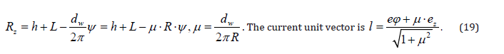
Let its winds number be equal to N so that to calculate the force one is to integrate upon ψ from 0 to 2πNw The calculation results are shown in the Figure 5. As it is seen, the solenoid behavior sufficiently differs from the wind’s one. Besides evident rise up of all forces modules due to the winds summation (proportional around to Nw) there are sign change of the Lorentz azimuthal force and axial forces inequality below the central plane. These asymmetries may be generated by the ab-sence of current closure mentioned above. The more detailed analysis is needed including the bi-filar wending and trajectories’ calculation to understand properly the solenoid case.
And once again, as in the previous case, it’s worthwhile to emphasis the principle difference between the alone wind and solenoid currents’ interaction with a probe charge. If the Huygens model is essentially true, the theory of many ion devices using the magnetic field, Penning sources among them, needs the revision. Precisely, the well-known “diocotron instability” may hardly be properly interpreted without the presumption of the magnetic field interaction with an immobile charge. Of course, they usually put permanent magnets inside such devices. Still, the theory of these magnets according to the Huygens principle is the subject of another, enormous research.
The infinite length straight currents interaction
As it has been noted in the end of the 2nd section, to choose between “the Huygens model” and the “full Huygens model” on is to consider the infinite currents interaction. The total attraction of the infinite length active unit current (1A) of the probe unit length (1m) infinite parallel unit current at the unit distance (1m) is equal to 2*10-7N (SI) according to the definition of 1A. That is:

As previously one is to sum the contributions of all charges interactions dFH=dF++dF−−+dF−++dF+− expanded and in β Maclaurin series with the accuracy of linear terms and where the zero term (ε ,∈= 0) is zero (dF++=0) The “full Huygens model” force element 1st term instead of (13) looks like(the factor (1−β2) is omitted due to its smallness):
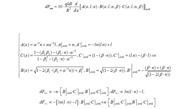
So, the total force element is equal to:
The final step is Maclaurin series expansion in φ =∈ξ with the accuracy of linear terms:
The “Huygens model” expression looks like:
The Cartesian frame is suitable in this case instead of the cylindrical one.
Let x – be the acting current element abscissa value, ξ – the probe current element abscissa value. Denoting l and ξ the currents’ unit vectors (i = l =ξ in this particular case) one may immediately write scalar and vector products of (5):
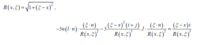
After integration 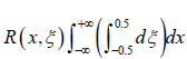 the normal (j) component of the Huygens model is equal to – 2 that is equal to the Lorentz one, whereas the full Huygens model normal component is – 4, that is twice larger. The tangential
(i) components for the parallel currents are zero. Thus, the “full Huygens model” must be rejected, at least for currents
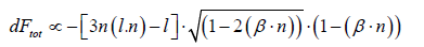
interaction. The Huygens model total force’s element is equal in the general case to:
the normal (j) component of the Huygens model is equal to – 2 that is equal to the Lorentz one, whereas the full Huygens model normal component is – 4, that is twice larger. The tangential
(i) components for the parallel currents are zero. Thus, the “full Huygens model” must be rejected, at least for currents
interaction. The Huygens model total force’s element is equal in the general case to:
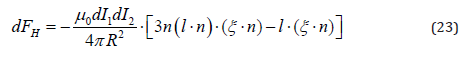
It may be compared with the Ampère force:  for different cases,
still it will be done elsewhere. Still, the final expression (23) may be written as:
for different cases,
still it will be done elsewhere. Still, the final expression (23) may be written as:
Conclusion
i. In order to understand many “magnetic field paradoxes” the Huygens principle model has been considered. Its important
aim is the replacement of the “field description” by the purely geometrical approach.
ii. This approach is rather easy to realize in the case of free charges and currents. One need not to calculate the magnetic
field from the known current distribution or charges motion that is use the differential operators such as grad, div, rot.
The equations of motion may be immediately written according to the evaluated formulas.
iii. These formulas for the Huygens model give the proper result in the case of the parallel currents attraction. However,
the full Huygens model gives more reasonable formulas in the case of arbitrary moving charges. Perhaps, it is due to
larger relative speeds. Still, none of these models is sufficient to describe the elementary charges interaction.
iv. 4. The “magnetic field work” certainly exists, at least for the interaction of an infinite current and a free charge.
Though, it is hardly possible to write the Lagrange function or canonical equations according to the Huygens model
regardless the used model.
v. Some experiments – mental and physical – are proposed to check the Huygens model’s predictions. The observation
of evaluated simplest forces results – the straight current, wind and solenoid interactions with the arbitrary moving
probe charge may be considered as physical, though the evaluation itself is certainly mental.
vi. In the case of the Huygens model justice (even partly) the theories of different phenomena are to be revised. Z-pinches
and Penning cells diocotron instability are among them.
vii. The described model is not suitable to permanent magnets yet. It is very complex research that may be accomplished
only by the rather large team.
There rest some interesting aspects of this model which will be investigated in the nearest future.
References
- NN Schitov (2024) The Maximum Principle and the Charge’s in the Electromagnetic Field Canoni-cal Equations // Applied Sciences Research Periodicals pp. 112-119.
- NN Schitov (2025) To the Question of a “Magnetic Field Work” // Applied Sciences Research Peri-odicals pp. 162-174.
- NN Schitov (2011) Relativity in Maxwell’s Electrodynamics. Part I, Фотоника (FRos) p. 56-61.
- NN Schitov (2013) Relativity in Maxwell’s Electrodynamics. Part III, Photonics p. 92.
- W Ritz (1911) “Gesammelte Werke”, Paris pp. 317 – 426, “Sur l’electrodynamique generale”.
- LD Landau (1988) E.M. Lifshits. The Physics Theory: manual in 10 vol. Vol. II The Field Theory p. 69-71.
- JD Jackson (1962) Classical Electrodynamics, Copyright © by John Willey & Sons, Inc. New York.
- IE Tamm (1976) The Electricity Theory Basics pp. 207.


