Review Article

The Heterogeneity Minimum Principle

NN Schitov*

Dukhov Automatics Research Institute (VNIIA), 22 Suschevskaya Ul., Moscow 127055, Russia

Submission:February 18, 2025; Published:March 11, 2025

*Corresponding author:NN Schitov, Dukhov Automatics Research Institute (VNIIA), 22 Suschevskaya Ul., Moscow 127055, Russia

How to cite this article:NN Schitov. The Heterogeneity Minimum Principle. Paper Recycling Ann Rev Resear. 2025; 12(4): 555841.DOI: 10.19080/ARR.2025.12.555841

Abstract

The new variational principle concerning continuous medium is proposed. As applied to mechanics and field theory it’s the native generalization of the optical-mechanical analogy whereas with reference to transport phenomena – it generalizes to 4D continuum the well-known Prigogine theorem concerning the minimum entropy generation in steady state.

Keywords:Variational principle; Prigogine theorem; Entropy generation; Euler equations; Optical-mechanical analogy, Heterogeneity

Abbreviations:PLA: Principle of Least (stationary) Action; PLC: Principle of Least Constraint;

Introduction

Variational principles that are so widely applied in mechanics, with reference to continuous medium are practically undeveloped. In mechanics the dynamic systems behavior is described by the Euler equations (Newton’s or Einstein-Poincare) of the proper variation problem (e.g. D’Alembert-Lagrange principle or the Principle of Least (stationary) Action (PLA) in the Hamilton or Jacobi form) [1,2]. Another variational principle to which correspond not Newton’s equations, but the Appel’s ones is the Gauss Principle of Least Constraint (PLC) and in which by analogy with kinetic energy the “acceleration energy” is implemented. In both cases the square of the particle’s coordinate time derivative is minimized – in the PLA 1st derivative – kinetic energy, whereas in the PLC – 2nd derivative – acceleration energy [1]. The Hertz principle or the “trajectory curvature minimum” stated in his “Mechanics principles” is also known. The variational principles multitude is the consequence of the multiversion motion description, but: “As Gauss himself marks, every new principle brings the new viewpoint on nature laws” [1]. In all cases the 1D functional – the time integral is minimized. The corresponding Euler equations solutions give coordinates and velocities of system’s particles as time functions.

But if it is the question of 4D functions the generalization is made for the PLA too, that is for the particles motion description in different fields. However, at least two of Maxwell’s equations are also derived from this principle. A question is bound to arise: is the developed formalism specific to the field theory and relativistic dynamics or it may be generalized to other phenomena description? One can put the question otherwise: is there some more general variation principle which case is PLA? What does the Euler equation of the variation problem corresponding to this general principle looks like? From the historic viewpoint it should be noted that the first variational principle of physics problem – the light propagation in media with changing refractive index – is the Fermat principle. It by-turn is the generalization of the known Heron’s light reflection principle, based on the statement that nature acts by the most accessible and easiest ways [1] As applied to the light it means that its real propagation path needs the minimal time as compared with other paths between the same points. Klein [2, p.237] has noticed: “Thus the Fermat’s PLA surprisingly simply transforms into the “quickest arrival principle”. It’s necessary to understand what the easiest and most accessible nature ways are as applied to other phenomena.

The Prigogine theorem

In the transport phenomena problems-heat, diffusion or chemical reactions (disturbances locally transmitted) in the 3D continuum the Prigogine theorem of minimal entropy generation in steady state [4] is some analogue of the general variational principle. But only stationary transport phenomena equations – uniform or nonuniform elliptic equations as well as Helmholtz ones follow from it. The volume density of entropy generation is determined as the sum of scalar products of thermodynamic flows Ji and thermodynamic forces X_k. The variables gradients determining the system’s state, e.g. temperature gradient, are thermodynamic forces. In the linear nonequilibrium thermodynamics, one of which basic statement is the Prigogine theorem, the linear dependence of flows upon the forces is implied: (linear phenomenological laws). Thus in the continuous media physics the state variables gradients play dual roles – flows and forces linearly bound. As a result, for systems without chemical reactions and viscous friction the division on the terms analogous to the “kinetic” and “potential” energies is impossible. Coordinates are the problem’s arguments and cannot be state variables. (At elasticity description the state variable is really the length dimension value – the displacement, but it’s the coordinate’s function itself.)

On account of linearity the entropy generation in a volume V without chemical reactions may be expressed as the volume integral with the sum of gradient squares as the integrand [4]:

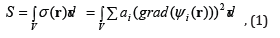
where ψi – Plank potentials – are state variables. Then the Euler equations of such a variation problem (the entropy generation minimization) represent the equalities to zero of corresponding flows divergences – the uniform elliptic equations. (See, however, the Appendix 1.)

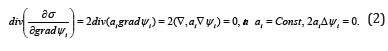
By analogy with mechanics, one would multiply the integrand in (1) (the entropy generation’s density) on ½ and call it the heterogeneity energy of state variables ψi. Thus, the general variational principle, describing the steady state of continuous media may be called The Heterogeneity Minimum Principle (HMP). Speaking like Heron one could say that nature seeks to smooth out the appearing heterogeneities. (From the statistics point of view such a statement is perhaps equal to the entropy increment.) At that as in mechanics the kinetic energy remains constant in the absence of external forces (free particles) in the continuous media (in the absence of chemical reactions and viscous friction) the “heterogeneity energy” density remains intact too. It may have an arbitrary but minimal value determined by boundary conditions. This minimal value may be zero in the general case because the Laplace equation (2) allows the solution in the form (see [8, chapter 10]):

where k may be complex. However, in the case of solution expression as the product of linear functions of Cartesian coordinates the heterogeneity energy density equality to zero is not so obvious and is the object of the additional investigation.Were it not for this new conservation law one shouldn’t formulate the new variational principle in addition to the Prigogine theorem. Still in the case of chemical reactions the energy analogue is conserved too. Let’s mark that the dimension of this analogue doesn’t coincide with the energy density dimension but may be different for different phenomena. The theory of heat conduction and diffusion in systems with chemical reactions is mostly analogous to the oscillating systems theory. This analogy is reflected in Table 1 (the denominations are taken from [4]). The sum of state variables products with corresponding phenomenological coefficients describing chemical reactions is analogous to the potential energy in mechanics whereas to eliminate any confusion (see next section) it could be called “sources energy”. Such a name may be well-taken because these reactions describe the existence of state variables sources (sinks).

Just another heuristic aspect of the considered analogy consists of the following. The diagonalization of matrices aˆ,bˆ is quite analogous to the Lagrangian of oscillating systems normal reduction. In this case the Laplace (or Poisson) equations are replaced by the Helmholtz ones Δψ∗_i− Λiψ∗_i=f(v) (the f (v) (the is determined from the Navier-Stokes equation). The Λi correspond to eigenfrequencies. The difference reveals itself in different signs joining the two square forms. That’s why in the case of thermodynamics there may be exponential as well as periodic solutions. Taking into account the elderly expansion terms in the mass action law is quite analogous to the accounting of the oscillating systems anharmonicity. As well as in oscillating systems normal frequencies are superposed with the combined frequencies oscillations in the thermodynamic ones there appear additional terms containing linear combinations of Λi in exponents [4].

The 4D Prigogine theorem analogue

Let’s suppose that the same HMP is valid in the continuous media dynamic problems that contain time dependence. It doesn’t mean that the additional implementation in (1) time integration leading to the appearance of the entropy in the right part means the minimization of the entropy itself which increases in irreversible processes and is maximal in the equilibrium. It means only the assumption of some quantity’s heterogeneity smoothing out in space-time as well as the smoothing out of a spatial heterogeneity following from the Prigogine theorem. The only difference consists of the fact that besides the spatial heterogeneity the temporal one – half of the time derivative square – is minimized too. It’s clear that the addition in (1) supplementary terms changes its sense – it’s no more the entropy generation!

Besides, on the transition to 4D description the 4th coordinate (time) unit vector should be introduced imaginary according to the definition of the metric tensor 4th diagonal component in [3, p.478]: g₄=g⁴=(e₄,e₄)=(e⁴,e⁴)=−1 One may give another “naïve-heuristic” explanation: the time unit vector is always normal to space unit vectors: . (The space coordinates may be chosen affine that is without any detriment to description whereas the scalar product of any space component on the temporal one must be zero which is characteristic to the complex plane. Supplementary arguments in favor of imaginary time unit vector will be given later on.) Coordinates themselves as well as the volume element are real while the volume element being the measure is nonnegative too. Then:
- unit vectors,

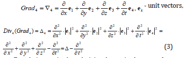
Exactly just as in the relativity theory in the case of constant coefficient a (speed) joining space and temporal coordinates it makes sense to introduce the new coordinate of length dimension by the equality. In this case the expression (3) acquires the casual form:
□а,

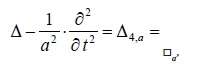
Where □а – is the common notation of the D’Alembert operator (D’Alembertian) for the speed “a”.

One should note at once that the 4D space is introduced in this particular case due to quite other reasons then Minkowski has made first [6]. In the case of continuous medium description, the imaginary time unit vector introduction arises from the unity of forms for static (3D) and dynamic (4D) variants. (If of course, the wave equation is universal in 4D continuum.) Minkowski has introduced the imaginary time for the interval invariance formulation convenience according to Einstein’s postulate. At that Minkowski 4-gradient which he has denoted “lor” is complex as in our case, whereas in [5] 4-gradient is real. The wave equation of continuous medium elastic oscillation [7] is also derived from the heterogeneity minimum principle with the substitution of scalar phenomenological coefficients by the tensor ones – the elastic constants tensor etc. This example illustrates the expediency of the heterogeneity energy density introduction instead of the kinetic and potential energy densities sum. In fact, in the pendulum oscillations description the elastic energy in the form of half product of rigidity coefficient on to the squared amplitude that is the state variable itself is named the potential energy. In the continuous medium the same elastic energy (in fact the energy volume density is meant but “density” is omitted everywhere for short) is the displacement and deformation tensors convolution. It is (in the isotropic case) the squared gradient which is closer in form to the kinetic energy [9].

Formally in this case too one can speak about the kinetic and potential energies because they are determined by different dimension constants: potential – by the elastic constant (for the longitudinal wave – Young modulus) with the dimension [N/m2]; kinetic – by density with the dimension [kg/m3]. However, after the division of the equation on to the elastic constant that is after transition to the symmetric (relative to coordinates) description the multiplier at the “kinetic energy” bilinear form instead of mass becomes a value inverse to a squared speed of elastic oscillations propagation. Describing the relation between Maxwell’s equations and MacCullagh’s theory F. Klein noted [2, p.286]: “By this the connection with the idea that potential and kinetic energies don’t present substantially different things and the difference between them is quite provisional is given”. The verily “continuous medium potential energy” may be only the bilinear form describing “chemical reactions” because it is the form of the state variables themselves, not their gradients.

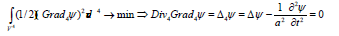
Thus, the 4D HMP gives (as the Euler’s equation) the uniform wave equation (written for one scalar state variable and one constant phenomenological coefficient for short):

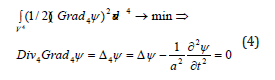
(See, however, Appendix 2.) At that the role of mass or the inertia measure plays the characteristic speed. The greater this speed – the less the system’s inertia, that is almost the tautology. From the form community of HMP follows that the wave equation (hyperbolic) conserves the heterogeneity as well just like the stationary one (elliptic). Simply this heterogeneity propagates at speed a. For the 1D wave equation fundamental solution [10] it would be the plane front behind it the state variable constant value is conserved, whereas in the 3D case – the spherical infinitely thin front (- Heaviside function, unit step):

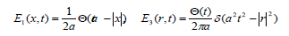
The heterogeneity in the initial moment concentrated in the origin smoothing out occurs (in the 1D variant) in the form of its propagation on to the whole space at speed a. In other words, inside the heterogeneity propagation front the space is uniform with constant value of the state variable which heterogeneity propagates. In the 3D variant the heterogeneity smoothing out occurs by the spherical infinitely thin front propagation. The variable surface density decreases in this case inversely proportional to the front’s surface – sphere’s surface – the Coulomb law in some sense. In this case inside the front the space is also uniform but with the state variable equal to zero. It is clear that 1D variant is the idealization whereas 3D corresponds to real matter. The arbitrarily small value of heterogeneity density is reached at the finite time determined by the propagation speed. Naturally the spherical fronts superposition – the Huygens principle – corresponds to the source wise representable real source of heterogeneity, that is every point of the source is the center of the heterogeneity propagation spherical front. In the 1D and 2D cases due to the absence of the descending part occurs the wave diffusion [9].

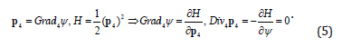
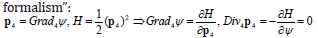
For the 3D vector V the minimization of its squared 4-gradient which is a second-rank tensor also leads to the wave equation (4) with the accuracy to the substitution of a scalar on to a vector. Turning back to analogy with mechanics let’s note that the transition to the “canonic formalism” is obvious:

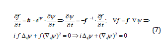
The eikonal equation

In the 1D case the solution of wave equation (4) – a plane wave being substituted in the 4-gradient expression gives (at ):

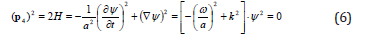
This equation is well known – the eikonal equation if ψ is the phase, not Plank’s potential as in (1). As it’s seen not only phase but the solution itself in the case of plane wave satisfies the eikonal equation. Besides, not only the equation but the solution has exactly the same form as 3D one, precisely:

Thus, being applied to optics the Euler equation really gives as a solution the function (plane wave in the space uniformly case) minimizing the 4-gradient square though its minimum is zero. It is an auxiliary argument in favor of the imaginary time unit vector introduction: the temporal heterogeneity compensates for the space’s one so that their sum is zero. By this a possible uncertainty of a conservative value magnitude in the case of 3D continuum at the transition to 4D one is eliminated – the value is zero. But the phase itself mustn’t obligatory satisfy the wave equation. In [5] the eikonal equation is obtained through the phase expansion in Maclaurin series and the limit transition concerning the wavelength converging to zero in the wave equation. It means the neglect of higher derivatives as compared with the squares of the first ones. In fact the wave equation solution in the form f (r,t) = a(r,t) ⋅ e^iψ permits one to evaluate the more precise equation which a phase satisfies. If one doesn’t neglect the second derivatives and implies (for simplicity sake) the amplitude constant: , then differentiating the solution and substituting in to the wave equation one gets:

Hence a phase (and correspondingly an action in the Hamilton’s mechanics) satisfies a complex equation, at that vanishing means simultaneous vanishing of real and imaginary parts. The real part vanishing is in fact the eikonal equation whereas the imaginary one – the wave equation. According to the eikonal value (or wavelength) one can imply zero either real or imaginary parts. The analogy with the quantum mechanics is obvious (see Appendix 3). Though, in [10, p.83] there is such a remark: “The substantiation of a passage to the limit from the wave equation to the eikonal one is in fact a very ticklish problem which is described in [21, 45 from 10]”.

The HMP relation with PLA

Thus, the wave equation is the Euler’s equation of the variational problem of the heterogeneity f minimization and its solution in the form of plane wave gives for the phase (action) the eikonal and wave equations. One may assume that not only action but its heterogeneity (equal to zero in the case of sources absence) too is minimized. But is it really so? Is HMP really applicable also to the action and will its heterogeneity be constant and zero (as in the case of eikonal) is far from being obvious. It’s known that the action 4-gradient may be presented in the form ([5, p.120]):

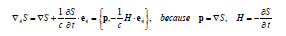
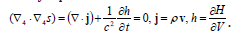
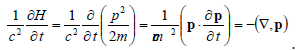
However, the action in mechanics is the time integer, not the 4D volume one. If just as in the field theory one assumes the action as the 4D volume integer then one must change the mass on to the density, impulse on to the flow density and energy on to its volume density. In this case the Euler’s equation for the density of the action – s – is as usually the uniform wave equation. Expressed in terms “flow density – energy density” it acquires the form of the continuity equation:

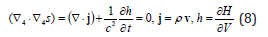
In this case it’s obvious that (after 3D volume integration) for the free particle H = E =mc² (with the accuracy to the Lorentz’ radical 1−β² in the denominator that is at the flow definition with the same radical gives the whole coincidence). Thus, the famous Einstein’s relation “from the HMP point of view” is the consequence of the definitions of 4D action gradient and impulse. So much the same the well-known relation p = Ev/c² is the consequence of the equation [8]. In the case of the absence of explicit dependency of the Hamilton’s function upon time (energy conservation) the impulse divergence vanishes – the incompressible medium. If the divergence isn’t zero, the energy decreases at positive divergence and vice versa. It may be interpreted as the energy decrease in a given volume due to particles leaving off this volume and increase in the case of new particles arrival (mass increase in this volume). If the transition from a density to an action by 3D integration is correct the free particle action heterogeneity in the relativistic approximation looks like:

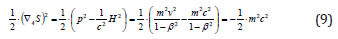
It’s seen that the action heterogeneity is constant, probably minimal, but not zero. If one takes not half but entire squared action’s 4-gradient – 4-impulse, then one gets (with the accuracy to the sign) the well-known SRT result: the squared 4-impulse is constant and equal to m2c2. We should note at once that the 4D Hamiltonian is just equal to the half of the squared action’s 4-gradient (see (9)) that is not precisely the same as the squared 4-impulse in SRT. The 4D generalization of a Hamiltonian looks quite more natural compared with the 3D one: if in the 3D case the free particle’s Hamiltonian is equal to the half of the action gradient divided by the particle’s mass in the 4D one it’s simply the half of the 4-gradient square. Still, it becomes negative and to conserve the precedent logics demanding it’s vanishing one should add to the Hamiltonian the half of the “rest 4-impulse” square equal to 1/2m²c². However, such an assumption needs a serious analysis and is beyond the frame of this work. Perhaps it’ll be better to minimize −1/2(∇₄S)² having in view that an integrand must contain the positive source function providing the mass existence. In the case of its absence the heterogeneity smooths away (vanishes) due to the “mass flowing out” of a given volume.

In fact if the minimized function is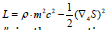

then H = m²c² . We need “the chemical term” in the equation (8):

(Appendix 5).

The continuity equation, relation with electrodynamics

Hence in the general case the 4-vectors containing temporal component introduction the HPM Euler’s equation (wave equation) acquires the auxiliary sense of the continuity equation (the strict balance equation [4]):

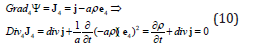
Here а – some characteristic flow speed:

the density or concentration of the corresponding component). At that for а = Const the squared gradient vanishes in the whole 4D space that is it’s conserved and minimal:

This fact is another one supplementary argument in favor of imaginary time unit vector introduction.

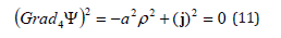
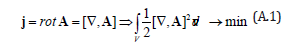
Being applied to electrodynamics, the equation (10) acquires another sense too. If the electromagnetic field’s 4-gradient is the 4-gradient of some scalar Ф then the Euler’s equation of the variational problem of this scalar squared gradient minimization is the Lorentz gauge [5] and at the same time the uniform wave equation for (see Appendix 4):

The Ф dimension is easily determined from its 4-gradient expression:

where q – is a charge. It’s quite another matter that 4-potental of an electromagnetic field cannot be equal to a some scalar 4-gradient because in this case the field tensor – the antisymmetric part of a 4-potential’s 4-gradient [5, p.244] identically vanishes in the case of differentiation’s order independence

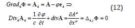
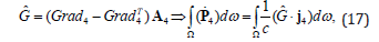
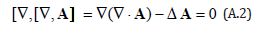
(in the 3D case it means the gradient’s curl identical equality to zero). But also in the general case of a 4-gradient presentation as a sum of a scalar’s 4-gradient and 4-divergence of 4-vector’s 4-gradient the Lorentz gauge is conserved (see (A.4) formulae for 3D case). At last if a density is the charge’s density (ρ_q) and a flow density is the electric current’s density (j_q) then the continuity equation is the Euler’s equation of the variational problem of scalar “F” heterogeneity minimization:

The dimension of the scalar I whose 4-gradient is the 4-vector of the current density is the potential in a unit time. If one minimizes the 4-potential’s heterogeneity, then one gets the uniform wave equations for the potentials as the Euler’s equations:

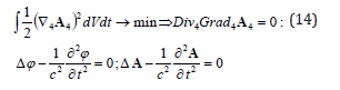
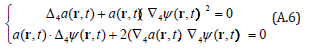
Equations (14) would become inhomogeneous if one accounts the second term in the charge-fields action considering the charges interaction in the exterior field (compare [5, p. 188]):

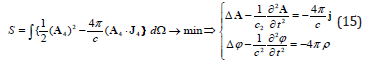
The system (15) may be rewritten using the scalars :

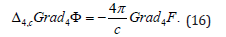
Due to the commutativity of the scalar and vector operators Δ₄ ,∇₄ from (16) follows

Hence we’ve come to the contradiction: due to the Lorentz gauge such equality mustn’t be valid (Appendix 6), still it is. Does it mean that Lorentz gauge isn’t true or the reason of it is in something else – the answer will be given in another article specially deduced to the electrodynamics. So one may say that Maxwell’s equations in the potentials wave equations form (in the absence of charges and currents) (14) are Euler’s equations of the variational problem of the 4-potential’s heterogeneity minimization. Or, taken separately, scalar and vector potentials heterogeneity minimization. Nevertheless, equations (15) are the Euler’s equations of the variational problem of an action minimization, not its heterogeneity being only part of this action. Is it possible in this connection to say that the HMP is more general principle? Apparently it is, at least for terms being squared space derivatives of 4D continuum. (Compare, for example, the substantiation of the free particle Lagrange function given in [5, p.17] with the general requirement of the heterogeneity minimization.) One can consider the scalar product of the potential and current density 4-vectors in (15) as the characteristic of the medium in which this heterogeneity is minimized. This medium simply contains sources and sinks of the function which heterogeneity is minimized. By what else these scalars are connected? They are connected through the charge in the field motion equations. At that the transition from densities to charges is made as usually by the 3D volume Ω integration:

where - is the 4D pulse’s density. In fact, from the definitions:

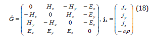
the charge in the field motion equation follow after volume integration:

and the energy balance equation

In the mechanics of continua [7], the antisymmetric part of the distortion tensor is named the small rotations tensor, whereas the symmetric one – the deformation tensor. Klein describing the McCullagh’s theory considers exactly the symmetric part of the distortion tensor as a tensor, whereas the antisymmetric part – the curl – as a vector. In fact, wave equations are obtained regardless of the presence in the variational problem the distortion tensor or only its antisymmetric part. Does the Euler’s equation [8] (Lorentz gauge) mean in this case (by analogy with the mechanics of continua) the field’s rigidness in the 4D sense or simply the absence of 4-potential sources? In what sense may the HMP be applied to the particle’s behavior description? It’s natural to call for getting ordinary expressions at the transition to point or at least having a finite volume object (Appendix 7). In fact, let the probability density of a particle existence in an elementary volume of 4D continuum is. In the external forces’ absence, the minimization of this density heterogeneity gives the wave equation with some unknown speed. But if this density is localized (to be more specific concentrated in the sphere of radius R situated in the moving point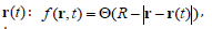

, then the 4-gradient degenerates into:

The squared 4-gradient after 3D volume integration takes in this case the form of the free particle’s action.

Conclusions

Omitting the section “Discussion” just because all above text is controversial or debatable (at least) let us enumerate some conclusions.
1. The new variational principle called “The Heterogeneity Minimum Principle” (HMP) concerning continuous medium is proposed. It is the attempt to generalize the known Heron’s statement: the nature acts by the most accessible and easiest ways. As applied to mechanics and transport phenomena it generalizes onto 4D continuum the well-known Prigogine theorem concerning the minimum entropy generation in steady state.
2. By analogy with mechanics the entropy generation’s density in the absence of chemical reactions and viscous friction Σ▒ 〖a_i (grad(ψ_i (r)))^2 〗 multiplied on ½ is called the heterogeneity energy of state variables . Thus the general variational principle, describing the steady state of continuous media may be called The Heterogeneity Minimum Principle (HMP): the nature seeks to smooth out the appearing heterogeneities. The Euler equations of such a variation problem (the entropy generation minimization) represent the equalities to zero of corresponding flows divergences – the uniform elliptic equations. As in mechanics the kinetic energy remains constant in the absence of external forces (free particles) in the continuous media the “heterogeneity energy” density remains intact too.
3. In the case of chemical reactions the energy analogue is also conserved just as in the oscillating systems theory. This analogue contains the sum of state variables products with corresponding phenomenological coefficients describing chemical reactions that is analogous to the potential energy in mechanic oscillating systems and could be called “sources energy”. In the linear approximation it looks like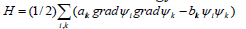

. Taking into account the elderly expansion terms in the “mass action law” is quite analogous to the accounting of the oscillating systems anharmonicity.
4. Being applied to 4D space-time HMP means only the assumption of some quantity’s heterogeneity smoothing out in space-time as well as the smoothing out of a spatial heterogeneity following from the Prigogine theorem. The only difference consists of the fact that besides the spatial heterogeneity the temporal one – half of the time derivative square – is minimized too. the addition of supplementary terms changes its sense – it’s no more the entropy generation. On this transition the 4th coordinate (time) unit vector should be introduced imaginary according to the definition of the metric tensor 4th diagonal component
5. The Euler equation of the 4D gradient square is the wave equation:

Applied to the continuous medium elastic oscillation this equation is also derived from the HMP with the substitution of scalar phenomenological coefficients by the tensor ones – the elastic constants tensor etc. The description analogy to the general relativity is obvious as well as the transition to the “canonic formalism”:

6. In the 1D case the solution of wave equation – a plane wave being substituted in the 4-gradient expression gives (at k=ω/a) the eikonal equation if ψ is the phase, not Plank’s potential. As it’s seen not only phase but the solution itself in the case of plane wave satisfies the eikonal equation. Besides, not only the equation but the solution has exactly the same form as 3D one. Thus being applied to optics the Euler equation really gives as a solution the function (plane wave in the space uniformly case) minimizing the 4-gradient square though its minimum is zero. The wave equation solution in the form f (r,t) = a(r,t) ⋅ e^iψ permits one to evaluate the more precise equation which a phase satisfies accounting the second derivatives. Hence a phase (and correspondingly an action in the Hamilton’s mechanics) satisfies a complex equation, at that vanishing means simultaneous vanishing of real and imaginary parts. The real part vanishing is in fact the eikonal equation whereas the imaginary one – the wave equation. According to the eikonal value (or wavelength) one can imply zero either real or imaginary parts. The analogy with the quantum mechanics is obvious.

7. Concerning the HMP relation with PLA it’s useful to recall that the action in mechanics is the time integer, not the 4D volume one. Generalizing on 4D one must change the mass on to the density, pulse on to the flow density and energy on to its volume density. In this case the Euler’s equation for the density of the action – s – is as usually the uniform wave equation. Expressed in terms “flow density – energy density” it acquires the form of the continuity equation:

In fact, it needs “the chemical term” (the positive source function providing the mass existence) in the right part: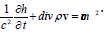

.

8. Being applied to the electrodynamics the continuity equation acquires another sense too. If the electromagnetic field’s 4-gradient is the 4-gradient of some scalar Ф then the Euler’s equation of the variational problem of this scalar squared gradient minimization is the Lorentz gauge and at the same time the uniform wave equation for:

The Ф dimension is easily determined from its 4-gradient expression and is equal to the electric charge. Note that 4-potental of an electromagnetic field cannot be equal to some scalar 4-gradient!

9. The electric charge continuity equation is the Euler equation of the another scalar F which dimension is the potential in a unit time. Minimizing the electromagnetic field 4-potential’s heterogeneity one gets the uniform wave equations for the potentials as the Euler’s equations. They would become inhomogeneous if one accounts the second term in the chargefields action considering the charges interaction in the exterior field (potentials wave equations at charges and currents presence). They may be rewritten using the scalars Φ,Ι : Grad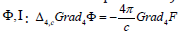

Equality being the consequence of the commutativity of the scalar and vector operators contains contradiction. It will be discussed in some other article like other interesting consequences of the HMP application in electrodynamics. To finish with let us emphasize that only the mathematical aspect of variational principles development has been briefly described. As for the “generally philosophic” aspect, it is the “eternal” problem (see Klein [2]).

Appendix

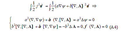
1. However, equality to zero of the flow’s divergence permits another solution, precisely the curl’s one, that is the flow is equal to the curl of some vector. In this case the heterogeneity minimization would mean the minimization of the half of this curl’s square:

In this case the Euler’s equations would look like:

And in the case of this vector’s divergence vanishing we get once again the Laplace’s equation but now for the vector: . It’s interesting that the minimization of the same vector presented as the scalar or vector heterogeneity gives as the solution either vortex or potential field or at least the constant. At that any of the solutions not constant is the necessary condition for alternative flow’s presentation – in the form of scalar’s gradient or vector’s curl, that is the curl’s minimization means the field’s potentiality, whereas the gradient’s minimization means the vortex character of the field. However, there may be case of both presentation coincidence, that is there are vector which curls are equal to gradients of some scalars, for example [8, p.174]:

At least if the flow is presented in the general form that is as the sum potential and vortex fields , then the Euler’s equations at the minimization of the half gradient and curl squares separately :

In this case the flow is either constant or its potentials – scalar’s and vector’s – satisfy the Laplace equation. At the presence of sources, the potential flow’s part is described by the Poisson equation which fundamental solution gives for the flow the Coulomb law. By analogy the vortex part is described by Biot-Savart law (at the constant vector v).

2. Drawing an analogy with PLA we note that the integrand in (4) analogous to the Lagrange function coincides with the energy analogue (the Hamilton function with the accuracy to redenomination through generalized pulses) as well as the free particle kinetic energy. At that the Euler’s equation solution minimizing the heterogeneity at the same time gives its constancy and equality to zero. Such a “conservation law” has hardly more universal nature than the energy conservation law. This law claims the time constancy of some scalar value at the predetermined circumstances at that this value may be different. Whereas from HMP follows that in the case of sources absence the heterogeneity of any value of arbitrary tensor dimension is minimal, constant and equal to zero in the 4D continuum area where it has been “smoothed out”. It’s singular on the propagation front (far the space wave, not plane or straight line due to the falling edge absence) and is zero at the both sides of this front.

3. What’s the frontier of this transition? To determine it one may probably set equal the second derivative to the squared first one. It gives for time derivative:

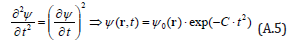
The analogous expression would be obtained for the space coordinates dependencies. If C is small than “the wave packet” don’t smooth out a long time and one may speak about the “point particle” motion.

In the opposite case the packet smooth rather quickly and we have a pure quantum situation.

But if the amplitude is not constant than we’ll get from the wave equation the system of equations for the phase and amplitude:

This system is hardly interpreted and it’s not clear at once whether it’s an Euler’s equation system of some variational problem.

4. From the comparison of (12) with the Lorentz gauge follows that at least dimensionally introduced scalars could be bound by the equality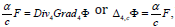

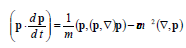
where α – the proportionality coefficient. But in this case I=0 due to the Lorentz gauge.

5. Writing the free particle energy in the nonrelativistic approximation we’ll get the following “equation of motion”:

If one transits to the full “substantial” time derivative according to the formula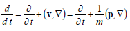

than one gets the following “equation of motion”:

6. At the same time the conventional (in the linear non-equilibrium thermodynamics) proportionality of the flow density to the gradient of this density (of opposite sign) (1) does not agree with the flow 4-vector presentation as the 4-gradient of some scalar (9). In fact, on this assumption this scalar is proportional to the density with opposite sign

∇Ψ = j = −D∇ρ ⇒ Ψ = −Dρ , that necessarily leads to the equation for the partial time derivative giving the exponentially increasing with time solutions:

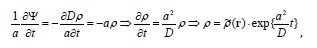
whereas the parabolic equations solutions decrease exponentially with time.

What’s the reason of such a contradiction? Has it some profound physical sense? What kind of equations – parabolic or hyperbolic (wave) describe the transport phenomena? The answers to these questions will be given in some other article. Meanwhile we simply mark the well-known fact of inadequateness of transport phenomena description (for example, thermos-conductivity) by parabolic equations implying the infinitely great propagation speed.

7. The continuity equation expression in the form of the flow 4-vector 4-divergence equality to zero (13, 15) is well-known (see, for example [2, 5]) and this claim hasn’t any particular value. However, recalling that it is the wave equation for a scalar which 4-gradient is the flow 4-vector (in the general case with the speed depending upon the 4D continuum point) one may make the absolutely new conclusion. If this dependence is known and boundary conditions are set one can routinely obtain the corresponding wave solution, e.g. in the form of plane wave. So then the 4-vector components – density and flow density being time and space derivatives would also have the wave form. It’s particularly important due to the fact that the Schrödinger equation is the continuity equation linearization (see [2, p. 497-501]). Thus, the denying of a particle point image and its substitution by the function distributed in 4D continuum inevitably leads due to the HMP to wave solutions. The same is possible in the case of point image conservation at the determined description by the probable one with the probability density distribution determined on 4D continuum – the quantum mechanics.

References

1. EN Berezkin (1974) The theoretical mechanics course, Moscow State University publishing house, Moscow, in Russian.
2. Felix Klein (1926) Vorlesungen über die Entwicklung der Mathematik im 19. Jahrhundert, Teil I, Berlin, Verlag von Julius Springer.
3. E Madelung (1957) Die mathematischen Hilfsmittel des Physikers, Berlin, Göttingen, Heidelberg, Springer-Verlag.
4. SR De Groot, P Mazur (1962) Non-Equilibrium Thermodynamics, North-Holland Publishing Company, Amsterdam 8: 10.
5. LD Landau, EM Lifshits (1969) The short course of theoretical physics. Book 1, Nauka, Moscow, in Russian.
6. H Minkowski (1983) Basic equations of electromagnetic processes in moving bodies, “Einstein’s collection 1978-1979”, Nauka, Moscow, in Russian. (In German: Grundlagen für die elektromagnetischen Vorgänge in bewegten Körpern.)
7. Yu I Sirotin, ML Shaskolskaya (1979) The foundations of the crystal physics, Nauka, Moscow, in Russian.
8. Granino A Korn, Theresa M Korn (1968) “Mathematical Handbook”, McGraw-Hill Book Company, New York San Francisco Toronto London Sydney.
9. VS Vladimirov (1976) The equations of mathematical physics, Nauka, Moscow, in Russian
10. VV Kozlov (1998) The general vortex theory, The Udmurt University publishing house, Izhevsk, in Russian.