Abstract

Following up with previous advance series, volumetric wear predictions for alloy-UHMWPE Total Knee Arthroplasty (TKA) are simulatedoptimized for classical Archard’s model (AM). Mathematical algorithms for Integer and Integral volumetric wear are explained. 2D-3D Imagingprocessing computational simulations software designed with Graphical Optimization and Interior Optimization techniques. For [1-5] Million Cycles (Mc) results in Volumetric Wear, the numerical dataset and 3D simulations image-processing graphs are demonstrated. Second part shows improvements-review for AM Linear Abrasion. Applications in Biotribology/Biomaterials are presented.

Key words:Total knee arthroplasty (TKA); 3D Simulations; Optimization; Linear Wear; Mathematical Model; Load; Sliding Distance; PE (Polyethylene); Wear Factor (WF)

Abbreviations:Archard’s Model: AM; FE: Finite Elements method; K_wear: Wear Factor (WF); L_wear: Linear, V_wear: Volumetric Erosion; Mc: Million cycles; PE: Polyethylene (UHMWPE); TKA: Total Knee Arthroplasty; UHMWPE: ultra-high molecular weight polyethylene.

Introduction and Objectives

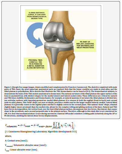
Continuing in UHMWPE-TKA prostheses research line, this study focuses on TKA volumetric abrasive erosion computational predictions. Linear and volumetric wear predictions show significant magnitude differences [1.1- 1.12, 2.1-2.32], Equations 1. TKA models are very specific as algorithmic-functions of, among others, anatomical, biomechanical, biodynamics, biotribological and bioenergy proper knee characteristics. Classically, Archard’s model (AM) formula applied for TKA wear is based, for linear wear, on a straight-line sliding magnitude of the femur TKA-alloy condyle along the UHMWPE tibial-part of the prosthesis, Figure 1. For linear AM, sliding distance is an important magnitude, but considering that within the algorithm, load can be divided by contact surface, it could result nonlinear, unless the pressure magnitude is directly implemented. AM do not consider the TKA shear phenomenon, and that is a biotribology inconvenient, [1.1- 1.3]. For AM, the linear and volumetric wear prediction calculations, consequently, differ in units and magnitudes, Equations 1-3. AM algorithm-constant is a dimensional so-defined Wear Factor with proper dimensions, (mm³ / N m)-note that for this study programming is set as (mm³/ N mm). Its magnitude order differs along the literature, around 10exp (-9, or -10) magnitude order, [2.3], provided is set as (mm³/ N mm). Fixed-bearing TKA and Rotatingbearing TKA show differences related to contact area [2.1- 2.7]. This is an important difference between two types of TKA-tibial-plateau component. Contact areas are different, but numerical linear wear predictions with AMs do not differ significantly. Unicompartimental TKA constitutes a different special TKA implant.

There are more differences between volumetric and linear wear and difficulties in their determination for TKA wear standards. One important characteristic of TKA along the extensive literature is the large variety of methods, biotribology laboratory apparatus, algorithms, units to present results, and ISO standards [2.6]. Here it is set the most important hurdles to understand and compare the amount techniques and results. The most frequently units to present results are mm/Mc for linear wear, and mm3/Mc for volumetric one. The wear magnitudes and rates differ in literature and laboratories for two main reasons: (1) the large variety of testing apparatus and methods, (2) the large variety to communicate/measure results. Namely, wear per Mc (mm), wear per year (mm), wear per Mc (mg), wear per year (mg), and others. When the study is in vivo, wear is usually expressed in mm/year, what is common is the polyethylene density approximately equal to water, about 0.96 mg/mm3. One reason for that is the archive of the patient history, that gives the number of TKA implantation years, and the wear of the implant is related to that lifetime. Additional complementary dataset and further reading can be found at [2.1- 2.7]. Conversion of units: although it seems complicated, some techniques can be used to convert undesirable units in any publication results into other ones more convenient if it is the case-approximately. When linear/volumetric results are shown in erosion/year, (it could be mm, mm3, or mg), there are references to calculate approximately the number of Million Cycles (Mc) per year [2.5]. In doing so, an approximation is got to convert mm/year into mm/Mc through statistics of average number of Mc per year [2.5]. For instance, if the results are shown in mg, it is easy to convert taking into account that UHMWPE density is approximately the water one, about 0.96 mg/mm3. ISO norms show kind of like hurdles to evaluate the literature results. ISO norms are regulated but profuse. When comparing experimental and simulation results/datasets it is rather difficult, even if the studies have set the same ISO norms, [2.6]. Different apparatus usage constitutes another difficulty. TKA biotribology laboratories use a large amount of different manufactured machines to get trustworthy results [2.5-2.6]. The apparatus differs in output units, design, or mechanical methods to measure erosion. As a result, it is a must to study all those before interpret linear or volumetric TKA erosion dataset. Finally, different computational methods and models are applied in the literature studies. The standard method for TKA erosion research is FE. However, the FE variety methods is large, and the algorithms implemented within FE calculations differ. The FE computational systems are varied, for example, Abaqus or Matlab, [2.1-2.7].

Therefore, the rationale of this study is to get an initial precise volumetric wear for UHMWPE TKA. AM is classical, but still widely used, (specially for FE calculations) and Cross-Shear model (not selected for this study), is more recent and in general gives higher erosion magnitude orders, e. g., [2.1-2.3]. It is not an objective of the research to assert any arguments to consider totally superior/inferior any of those models. Instead, the aim is explained and demonstrate AM algorithms, precision, predictions, and research options when using AM. What is biomechanically clear, Figure 1, is that the sliding of the TKA can be approximated, following AM, as straight line-curve, but anatomically it does not happen. The method used in Graphical and Interior Optimization software, with specific algorithms. The designed programming is precise and the graphs are intended be sharp and illustrative.

Objectives

Therefore, objectives are mainly two. First and foremost, to design software engineering for computational-simulations and optimization of volumetric AM. Secondly, to review and improve previous studies for AM linear wear. Complementary biomechanical and biodynamics applications are explained.

In summary, volumetric wear simulation-optimization research was done with the classical Archard’s model. Computational intelligence software was designed for AM algorithms. Improvements for AM linear wear were included. 2D-3D imaging-processing graphical and interior optimization results agree the most literature results for these models in linear wear. TKA applications are briefed.

Archard’s Model (AM) Volumetric Concepts and Algorithms

This section deals with the main AM algorithms for computational implementation. Mechanical parameters and units are detailed.

The Basic Integer AM Model Volumetric Algorithm

For TKA volumetric wear, an integer algorithm was developed based on AM, Equation 1. In the literature, several AM varied-algorithms have been presented [2.1-2.12]. Therefore, in this study, the basic volumetric algorithm-model from [2.3-2.11], applied and analyzed mathematically by Author, reads,

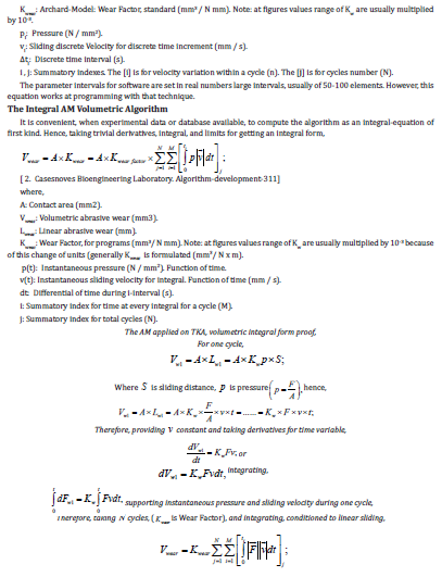
[ 1. Casesnoves Bioengineering Laboratory. Algorithm-development-311]
where,
A: Contact area (mm2).
V_volumetric: Volumetric abrasive wear (mm3).
L_wear: Linear abrasive wear (mm).
K_wear: Archard-Model: Wear Factor, standard (mm³ / N mm). Note: at figures values range of K_w are usually multiplied by 10^-3.
p_i: Pressure (N / mm²).
v_i: Sliding discrete Velocity for discrete time increment (mm / s).
Δt_i: Discrete time interval (s).
i , j: Summatory indexes. The [i] is for velocity variation within a cycle (n). The [j] is for cycles number (N).
The parameter intervals for software are set in real numbers large intervals, usually of 50-100 elements. However, this equation works at programming with that technique.

The Integral AM Volumetric Algorithm

It is convenient, when experimental data or database available, to compute the algorithm as an integral-equation of first kind. Hence, taking trivial derivatives, integral, and limits for getting an integral form,

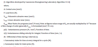
[ 2. Casesnoves Bioengineering Laboratory. Algorithm-development-311]
where,
A: Contact area (mm2).
V_wear: Volumetric abrasive wear (mm3).
L_wear: Linear abrasive wear (mm).
K_wear: Wear Factor, for programs (mm³/ N mm). Note: at figures values range of K_w are usually multiplied by 10^-3 because of this change of units (generally K_wear is formulated (mm³/ N x m).
p(t): Instantaneous pressure (N / mm²). Function of time.
v(t): Instantaneous sliding velocity for integral. Function of time (mm / s).
dt: Differential of time during i-interval (s).
i: Summatory index for time at every integral for a cycle (M).
j: Summatory index for total cycles (N).

The AM applied on TKA, volumetric integral form proof, For one cycle,

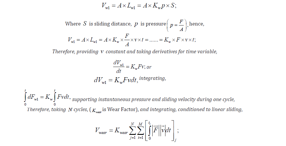
[3. Algorithm developed by Casesnoves Bioengineering Laboratory Algorithm 3114]
where,
A: Contact area (mm2).
F: Load force (N).
V_wear: Volumetric abrasive wear (mm3).
L_wear: Linear abrasive wear (mm).
K_wear: Wear Factor, for programs (mm³/ N mm). Note: at figures values range of K_w are usually multiplied by 10^-3 because of this change of units (generally Kwear is formulated (mm³/ N x m).
p(t): Instantaneous pressure (N / mm²). Function of time.
v(t): Instantaneous sliding velocity for integral. Function of time (mm / s).
dt: Differential of time during i-interval (s).
i: Summatory index for time at every integral for a cycle (M).
j: Summatory index for total cycles (N).

Computational Dataset and Methods

This section deals with units, dataset, and computational methods for the study with AM.

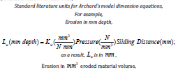
Volumetric Wear Units Precision

Equation 4 shows the physics units system implemented for AM simulations. The units were used for AM, that is N, mm3, and mm2. Then, standard TKA wear units read,

[4. Algorithm developed by Casesnoves Bioengineering Laboratory Algorithm 3114]
For volumetric AM, the second one is the primary method applied in this paper. That is Abrasive Volumetric Wear. Linear TKA knee-biotribology review/improvements are included at article second part.

Standard Abrasive Volumetric Wear Factor K_w Magnitude

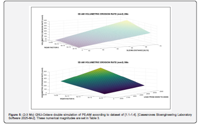
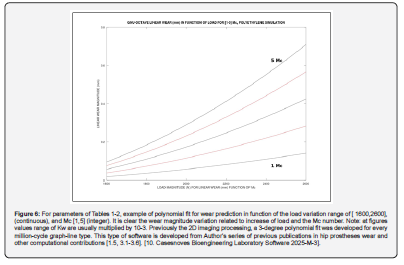
Given the fact that the number of laboratory apparatus, measuring systems, and hybrid studies are profuse, in the literature, there is not a total agreement for K_w wear factor magnitude [2.3]. Figure 2 shows a double plot for K_wand load related to Mc [1-5]. 2D GNU-Octave imaging processing multi-polynomial fit that describes the variation in function of K_w variation and Million Cycles (Mc) [2.13-2.21] integer interval. Note: at figures values range of K_w are usually multiplied by 10^-3. Figure 2-upper shows AM linear wear related to Load-Mc parameters for [1-5] Mc. Figure 2-lower 6 presents AM volumetric wear related to wear factor K_w for [1-5] Mc. Magnitude differences are significant.

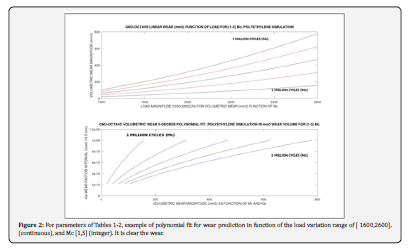
Figure 2 For magnitude variation related to increase of load and the Mc number. Previously the 2D imaging processing, a 3-degree polynomial fit was developed for every million-cycle graph-line type. [Casesnoves Bioengineering Laboratory Software 2025-M-3]. Also, for parameters of (Tables 1-2), example of polynomial fit for wear prediction in function of the variation range of [ K_w x 10^-3], (continuous), and Mc [1-5] (integer). It is clear the magnitude variation related to increase of [ K_w x 10^-3], and the Mc number. Note: at figures values range of K_w are usually multiplied by 10-3. Further references to contrast this dataset are generally in [1.1-1.12]. Previously the 2D imaging processing, a 3-degree polynomial fit was developed for every million-cycle graph-line type-different from upper Figure 2. This type of software is developed from Author’s series of previous publications in hip prostheses wear and other computational contributions [1.5,3.1-3.6]. [Casesnoves Bioengineering Laboratory Software 2025-M-4].

Computational Intelligence Dataset for Software

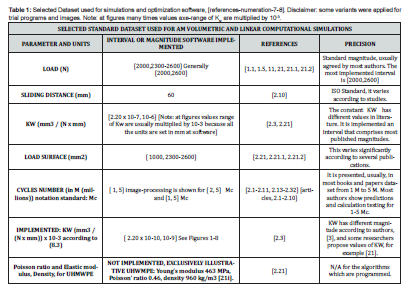
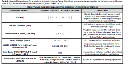
Dataset, (Tables 1-2), from literature is selected from parameter intervals at programs, because the commercial materials, TKA sizes, and Algorithm constants applied differ among authors, laboratories, testing apparatus, testing temperature, etc. As a result, it is necessary to choose those experimental datasets/magnitude-values which are commonly accepted in the literature. Therefore, the practical objective of the simulation-optimizations is to provide with large scale range that can be used to predict durability for all of those most important variants. Software is based on hip wear previous Author’s contributions for hip wear programming design [3.1-3.6]. In those publications, both Tikhonov Regularization Theory and Evolutionary Algorithms were applied for hip optimization software-engineering. General additional biotribology database can be found at [3.7-3.17].

Average Contact surface Magnitude

For volumetric wear, it is not necessarily needed for this kind of methods. That is a parameter interval rather difficult to implement within programs, both in Matlab and GNU-Octave. For both models in this study, the intervals published in [1.4] are set (Tables 1-2).

Benchmark polyethylene model (optional)

For volumetric wear, it is optional. There are variations for the TKA size in literature about laboratory studies. However, the size used for simulation software implementation was the most standard one, [2.1-2.3, 3.18]. That is, 78.2 x 44.2 mm the total coronal dimension, from that magnitude the contact surface was approximated-calculated. That size is according to ISO, and it is noteworthy to consider that there are ISO variants.

Sliding Distance (SD)

Sliding distance recommended by ISO is about 80 mm [2.10]. However, it was set [60,80] mm, taking into account differences between prostheses sizes, [2.12].

Load Magnitude Interval

This is a magnitude convergence point for most of studies. The most usual assumed magnitude by majority of investigations [2.21, 2.21.1-2.21.2]. For example [2.2, Table 2, page 63] gives an overview of the changes of loads and gaits from normal walk to down stairs/ramp. From this Table and setting a patient average weight of 75 kg, the interval of loads that comprise approximately walk, stairs and climb down/up, etc, can be deducted. Usually, then, is [ 1600, 2600] N interval. Here it is taken a maximum interval of [2000,2600] N in most simulation-programs. Other Authors, [2.21], apply a maximum load of 3000 N. That is not considered for this study, because those loads are not for usual patient walk. That is, walk to down stairs in a normal patient activity happens during a few minutes in general.

Standard Unit System

The Volumetric Wear standard TKA erosion AM units used in literature, most times, are mm3 of eroded material or mm depth of erosion along contact surface. When studies are in vivo or provided with cadaveric history, the Linear Wear is given in mm/year. It is not an objective of this study to discuss the optimal unit system. Instead, the image-processing and numerical data is expressed in mm3 volume to bring for user the choice to compare dataset appropriately, [2.3,2.11]. For passing erosion magnitude/year to mm3, it is taken into account the average Mc for a year, [2.16], which is about 2 Mc/ year-precisely, that is a rather difficult parameter since variations among patient groups, countries, and laboratories are high. The physics dimension equations for AM Linear and Volumetric Abrasive Wear are explained in Equation 4. Tables 1-2.

Volumetric Wear Dataset

Table 1 shows dataset implemented parameters for volumetric AM wear

Computational intelligence Software

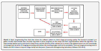
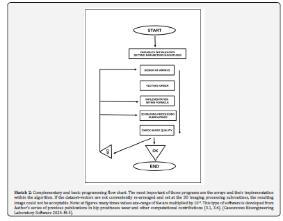
The most important parts of the software are mainly two. Both are difficult. The first one is the matrices setting withing patterns and their congruence for mathematical operations. The second hurdle is the 2D-3D imaging processing subroutines setting, because not any order for getting an accurate image is efficacious when obtaining the 2D-3D image.

Programming Structure

It was developed, Sketchs 1-2, software programming mainly from previous experience in hip wear models [2.33- 2.34]. Systems used were Matlab 2023 and GNU-Octave 8.1.0. For programming algorithms 1-2, the difficulty was the matrices congruency and the loops for arrays. Figure 3 shows the software pattern to check image-processing quality. Sketchs 1-2 explain the basic programming structure.

7 AM Volumetric Wear Results

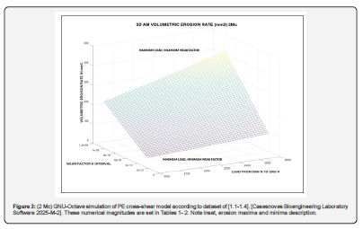
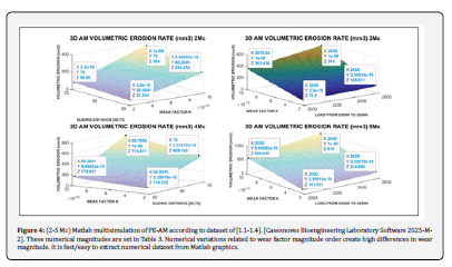
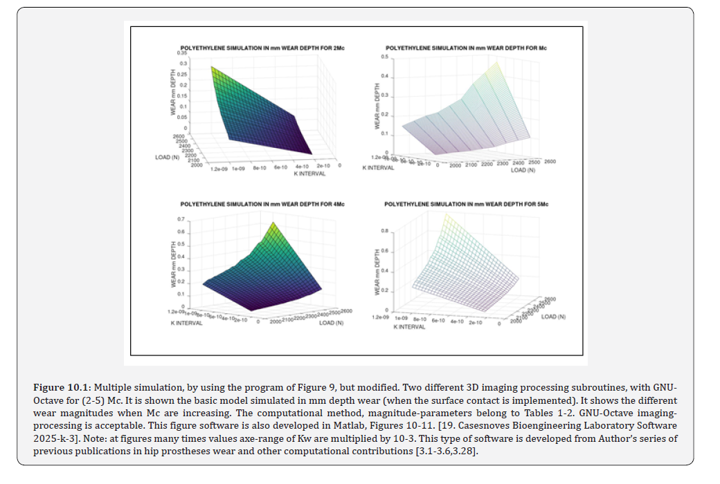
Figures 2-5 shows the AM volumetric wear for 2-5 Mc, GNU-Octave and Matlab imaging-processing system. Matlab image-processing quality and tools are better, but GNU-Octave is acceptable. The minimum Mc is chosen 2 because it corresponds approximately to 1 year erosion in literature, Table 2. However, this criterion, [2.16], is not completely confirmed in literature, and constitutes an approximation. Cycles number per year depends on multiple factors, e. g., activity, country, work, personal habits, sex, etc.

Volumetric Graphical Simulations Results

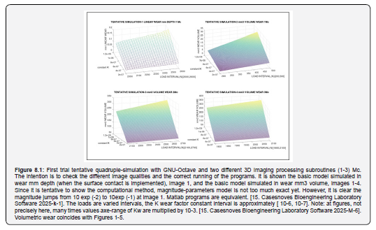
Graphical results with imaging-processing are set in Figures 2.1-6. Several software designs/subroutines were used to obtain all images.

Volumetric Numerical Results

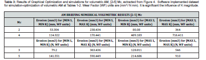
Table 3 shows the main numerical results for AM volumetric wear with load and sliding distance intervals, extracted from Figure 4. Results are presented in max-min four intervals. Namely [60,70] mm, and [2000,2600] N. The Figure 4 cursor numerical results are used to make the Table 3.

8 AM Improvements-Review Linear Wear

Linear Wear AM Concepts-Algorithms

Primary approximations are to consider exclusively the TKA wear, and exclude Creep and Lubrication Factors, (algorithms 5-8). Therefore, the calculations of this study part constitute the improvements/review of linear wear optimization-determination to get wear durability predictions of the TKA implant with fundamental physical formulation [1.5]. In the literature, variations of models are applied, e.g. [2.1, 2.4-2.6], although the most applied is Archard’s model with several variants. Basic measurements taken into account in this study section for in vitro and in vivo and contact area correspond to [2.1-2.21]. Typical values of TKA wear, most times obtained by FE method are referred at [2.18-2.32].

The basic Model algorithm(s)

The basic algorithm-model from [2.3-2.11], applied and analyzed/developed mathematically by Author, reads,

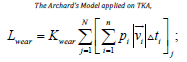
[ 5. Casesnoves Bioengineering Laboratory. Algorithm-development-311]
Where,
L_wear: Linear abrasive wear (mm).
K_wear: Wear constant, standard (mm³/ N mm). Note: at figures values range of K_w are usually multiplied by 10^-3.
p_i: Pressure (N / mm²).
v_i: Sliding discrete Velocity for discrete time increment (mm / s).
Δt_i: Discrete time interval (s).
i, j: Summatory indexes. The [ i] is for velocity variation within a cycle (n). The [ j] is for cycles number (N).

The Creep and Friction Factors

Creep

Although those factors are not applied in the study, description with details of the Creep and Lubrication formulas are conveniently shown. Creep equations are usually very similar for both models, Archard’s and Cross-Shear. For Creep, [2.3], the Archard’s model-equation format (Lee and Pienkowski, 1998) reads,

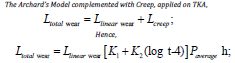
[ 6. Casesnoves Bioengineering Laboratory. Algorithm-development-311]
where,
K₁: Model Constant, [3]. Values for K₁ and K₂ are respectively, 3.491 × 10⁻³and 7.961 × 10⁻⁴.
K₂: Model Constant, [3]. Values for K₁ and K₂ are respectively, 3.491 × 10⁻³ and 7.961 × 10⁻⁴.
t: Time of load (minutes).
P_average: (N/mm²)
h: Polyethylene thickness (mm)

Friction

One common Friction Factor, set within the general formula is: [ 1+3 μ²] ½, [21], with values for UHWMPE of around [10^-2] magnitude order. This Friction factor multiplies linearly the general formula (1). At this stage, it is not applied in the study. Friction was not set at this stage because the friction value in this case is, approximately,

(1+3 x 0.072) ^0.5 = 1.0073, [ adimensional]

[7. Casesnoves Bioengineering Laboratory. Algorithm-development-311]

That is, a magnitude order of 10^-3. This implies that the magnitude difference if set within algorithms would not determine a magnitude order significance. That precision is useful for further refinements.

1.1. The Linear Wear Integral AM Algorithm

It is convenient, when experimental data or database available, to compute the algorithm in integral-equation of first kind. Hence, taking trivial derivatives, integral, and limits for getting an integral form,

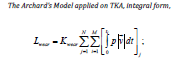
8. Casesnoves Bioengineering Laboratory. Algorithm-development-311]
where,
L_wear: Linear abrasive wear (mm).
K_wear: Wear constant, for programs (mm³ / N mm). Note: at figures values range of Kw are usually multiplied by 10^-3 because of this change of units (generally K_wear is formulated (mm³/ N x m).
p(t): Instantaneous pressure (N / mm²). Function of time.
v(t): Instantaneous sliding velocity for integral. Function of time (mm / s).
dt: Differential of time during i-interval (s).
i: Summatory index for time at every integral for a cycle (M).
j: Summatory index for total cycles (N).

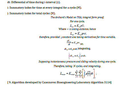
[ 9. Algorithm developed by Casesnoves Bioengineering Laboratory Algorithm 3114]

Abrasive Linear Wear Factor Kw Magnitude

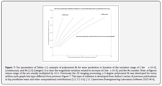
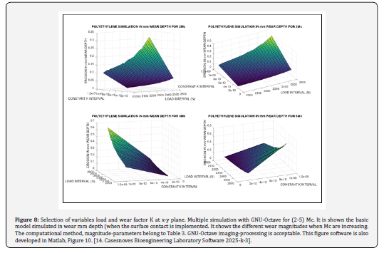
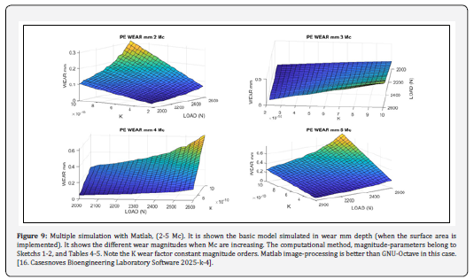
Given the fact that the number of laboratory apparatus, measuring systems, and hybrid studies are profuse along the literature, there is not a total agreement for K_w magnitude [2.3]. Figures 5-6 show 2D GNU-Octave imaging processing multi-polynomial fit that describes the variation in function of K_w variation and Million Cycles [2.13-2.21] integer interval. Note: at figures values range of K_w are usually multiplied by 10^-3. Figure 7 shows AM linear wear related to Load-Mc parameters. Figure 8 presents AM linear wear related to wear factor K_w from 1 -5 Mc. Tables 3-4.

Implemented Linear Wear Dataset and Units

The dataset implemented for linear wear is detailed at Tables 1-2, equivalent for volumetric and linear wear data. The units for AM linear wear are included in Equation 4. The software programming was developed mainly from previous experience in hip wear models and knee articles, [1.5,3.1-3.2,3.17]. Systems used were Matlab and GNU-Octave. For programming algorithm 5, the difficulty was the matrices congruency and the loops for arrays.

Computational intelligence Software

The most important parts of the software are mainly two. Both are difficult. The first one is the matrices setting withing patterns and their congruence for mathematical operations. The second hurdle is the 2D-3D imaging processing subroutines setting, because not any order for getting an accurate image is efficacious when obtaining the 2D-3D image. Figure 9 Program structures, as Sketchs 1-2, were developed software programming mainly from previous experience in hip wear models [2.33-2.34]. Systems used were Matlab and GNU-Octave 8.1.0. For programming algorithms, the difficulty was the matrices congruency and the loops for arrays. Sketchs 1-2 show the software pattern to check image-processing quality, explaining the basic programming structure.

9 AM Linear Wear Improved Results

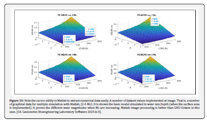
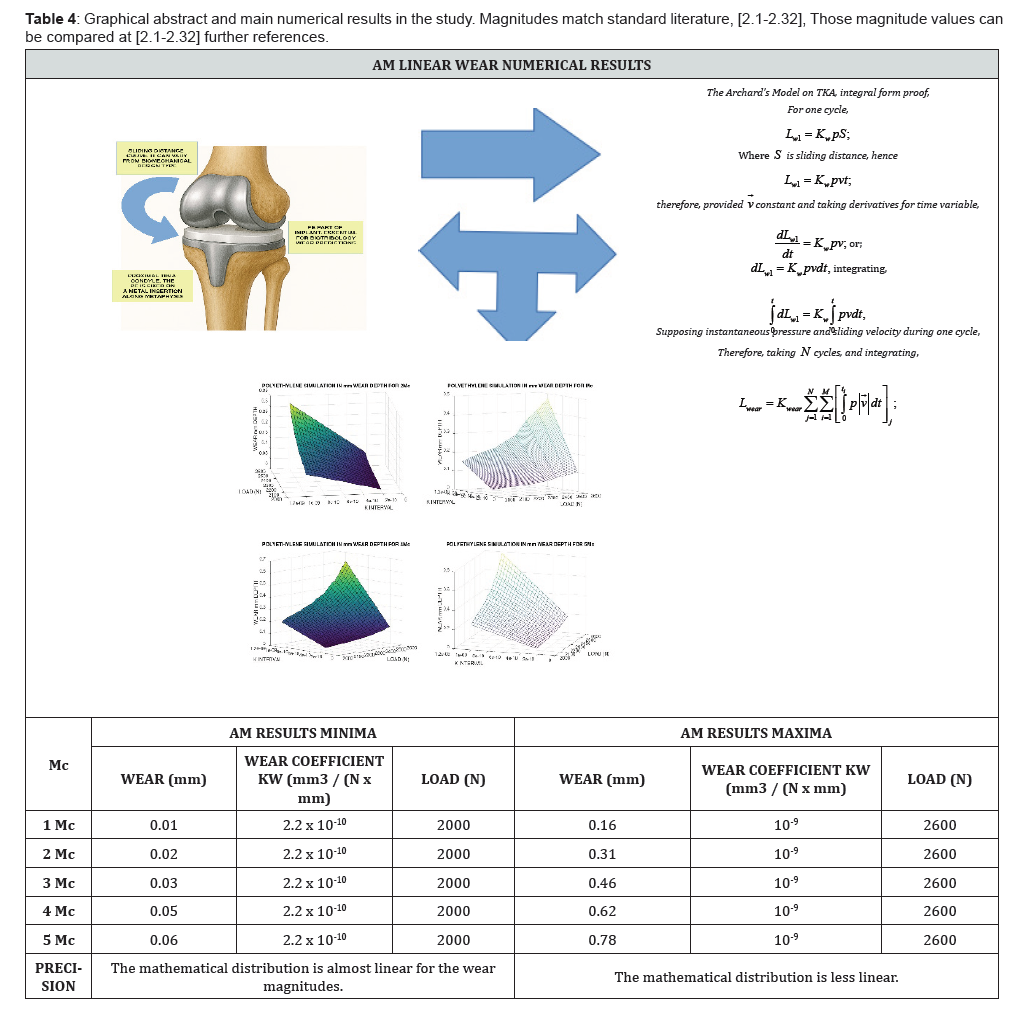
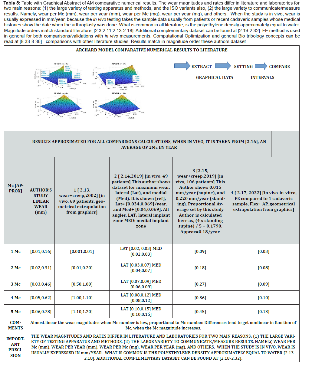
Results are divided into Graphical and Numerical. In this primary stage, the numerical ones were determined by Matlab graphical methods. Figure 10 The sharpness of 3D Graphical optimization is acceptable, and numerical figures show approximate coincidence with standard literature, Tables 4-5, [2.13-2.18]. Briefing of numerical comparisons to other Authors with Graphical Abstract are detailed in Table 5.

Graphical Optimization Results

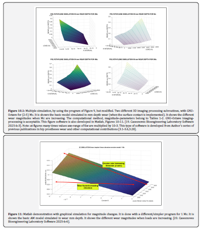
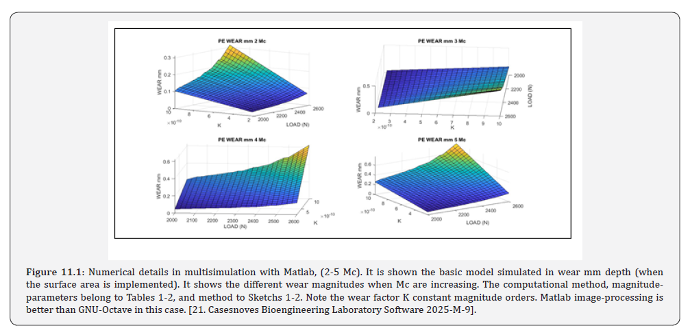
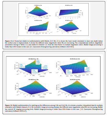
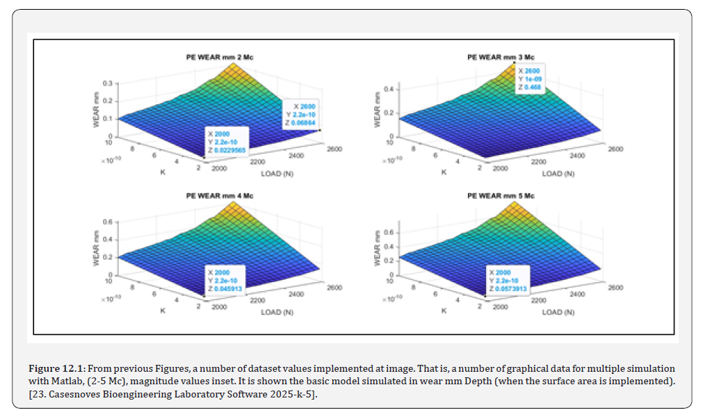
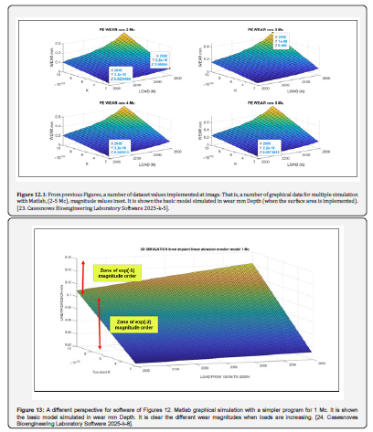
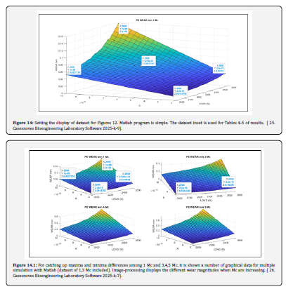
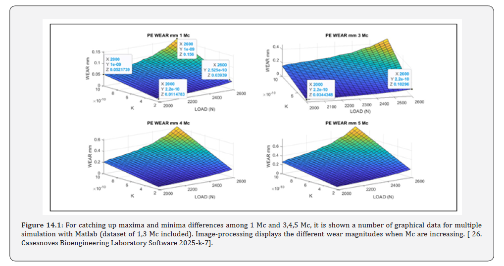
Graphical Optimization Method was developed during PhD Thesis and PhD Program publications, later in series of articles [1.5,3.1-3.2,3.17-3.28]. It essentially consists in finding the global/local minima by searching along the implemented 2D-3D imaging surfaces/curves of the algorithm objective function plus one/two selected parameters. Figure 11 Here it is applied on the wear formulas (3,6,8) to determine the optimal minima or any desired values subject to particular constraints along the 3D surface. In Ilustrative Example 1, it can be seen the process initiation. Firstly, some tentative programs are designed, after that, when checking the functionality of the software and the numerical congruence of the 3D graphs, the definite 3D Graphical Optimization Image-Processing charts are done with accurate parameters and intervals (Figure 12-14.1).

AM Linear Wear Numerical Results

Graphical Abstract within (Table 5) and tabulated magnitudes show extracted from Graphical Optimization the numerical data results for linear wear. Figures and magnitude orders match the standard literature. Those magnitude values can be compared at [2.1-2.32] further references.

Comparison of Numerical Results

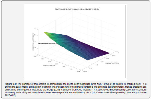
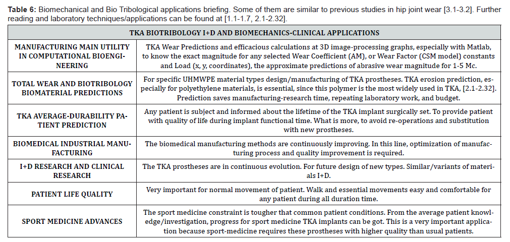
Graphical abstract within (Table 5) presents some numerical comparisons with other literature studies. Some of them are carried out with FE Method, others with FE Method and contrasted with cadaveric data. The most important objective consequence is that from [2,3] Mc on, the Linear Erosion shows a magnitude order jump from 10^-2 to 10^-1 mm. The comparisons are shown for database from [2.13- 2.17]. However extensive further database can be found at [2.18-2.32] (Table 6).

Discussion and Conclusion

The objectives of the research were two. First, to develop AM volumetric wear integer and integral equations. Secondly, simulate/compare the PE volumetric wear without creep AM predictions for TKA in a primary approximation. Complementary, an AM linear wear improvements from previous publications were included. Graphical Optimization for AM, numerical results, and comparison with literature dataset were presented. Some programming-recipes to develop simulation-software and an applications briefing were included. At this stage, Lubrication Factors for the models were not set.

Volumetric wear rates are primary results in this research, to be improved in next studies. The graphs obtained are acceptable and abrasive volumetric wear numerical results match approximately the standard dataset published, Figures 2.1-5, (Table 3). According to Table 3, the variation of volumetric wear related to wear factor is high. The higher wear factor, the higher volumetric rate variation in approximately exponential curves, Figure 2, Table 3. The calculated dataset at Table 3, from graphical optimization matches the published literature mostly [1.1-1.12]. Provided the wear factor value can be selected from graphics intervals Table 3, numerical dataset coincides approximately with other authors publications [1.1- 1.12]. The load shows be also a significant magnitude parameter for prediction calculations-at least one magnitude order. The higher load, the higher volumetric wear rate, Figures 2, 2.1-5, Table 3. Roughly speaking, the volumetric wear can be approximated from the linear wear multiplied by the magnitude order of contact area, Equations 1-3. This approach confirms the results of this study.

For 1 Mc AM abrasive linear wear is of the magnitude order [ 10-2, 10-1], and these predictions are more exact than primary volumetric findings. For Cross-Shear Type Models (CSM), [1.1-1.3], not included in this study, but softwarecalculated, the linear wear magnitude is higher, around 10 exp (-1) for 1 Mc. At linear AM in 1 Mc. at second review-part, the proven magnitude jump for this linear AM wear is presented as much clearly as possible, for instance, (Illustrative Examples 1-2).

It is significant, the rather strong influence of Wear Factor (WF) K in volumetric magnitude results, Table 3. WF magnitude varies according to authors actually, [2.3]. Numerical and graphical optimization results for AM volumetric wear match approximately the published ones. Advantages of this method related to FE technique are the fast results, and graphical visualization/comparison of results. Inconvenients are the software precision/equations developments that have to be checked. Another inconvenient is the matrices congruence arrange along program-patterns, both Matlab and GNU-Octave systems [3.29-3.45].

The image processing quality in GNU-Octave and Matlab is acceptable. It was tried to approximate/approach the most common numerical and graphical results published, given the large variety of variants for mathematical models-methods and ISO norms for TKA volumetric wear implants predictions.

In brief, a primary Graphical Simulations-Optimizations series for PE TKA implants abrasive volumetric erosion with AM were presented. Results for AM volumetric wear match approximately the literature figures and standards. Applications in Biotribology and Mathematical Optimization-Simulations are presented.

Scientific Ethics Standards

According to European Union and International Scientific Ethics [3.46-3.48]. All the software was done by Author. No Artificial Intelligence (AI) used for programming or any article-part, if wear so, it is declared, both in tools/systems for software anyway, and AI browsers-information. When any mathematical statement, algorithm/proposition/theorem is presented, demonstration and parameters/units are always detailed. Review of linear wear, algorithms and images, is selected from previous publications. If any inconsistency is found after publication, it is clarified in subsequent ones. When a citation such as [ Casesnoves, ‘year’] is set, it is to clarify intellectual property at current times, without intention to brag. The article is exclusively scientific, without commercial, institutional, academic, deliberate obfuscation, religious or religious influences, non-scientific theories, personal opinions, political ideas, or economical-conflict links. Author has no conflict of interest.

Author’s Biography

Dr Francisco Casesnoves earned the Engineering and Natural Sciences PhD by Talllinn University of Technology (started thesis in 2016, thesis Defence/PhD earned in December 2018, official graduate Diploma 2019). Dr Casesnoves is European Union and Internationally qualified as Doctor in Engineering to supervise PhD Theses, Master Theses, and Bachelor Theses in science and engineering. He works as independent research scientist in computational-engineering/ physics. Dr Casesnoves earned MSc-BSc, Physics/Applied-Mathematics (Public Eastern-Finland-University, MSc Thesis in Radiotherapy Treatment Planning Optimization, which was developed after graduation in a series of Radiation Therapy Optimization-Modelling publications [2007-present]). Dr Casesnoves earned Graduate-with-MPhil, in Medicine and Surgery [1983] (Madrid University Medicine School, MPhil in Radioprotection Low Energies Dosimetry [1985]). He studied always in public-educational institutions, was football player 1972-78 (defender and midfielder) and as Physician, supports healthy life and all sports activities. Casesnoves resigned definitely to his original nationality in 2020 for ideological reasons, democratic-republican ideology, ethical-professional reasons, anti-state monarchy corruption positions, and does not belong to Spain Kingdom anymore. His constant service to the International Scientific Community and Estonian technological progress (2016-present) commenced in 1985 with publications in Medical Physics, with further specialization in optimization methods in 1997 at Finland-at the moment approximately 100 recognized publications with approximately 65 DOI papers. His main branch is Computational-mathematical Nonlinear/Inverse Methods Optimization. Casesnoves best-achievements are the Numerical Reuleaux Method in dynamics and nonlinear-optimization [books 2019- 2020], The series of Radiotherapy Improvements for AAA superposition-convolution model, the Graphical and Interior Optimization Methods [2016-8], the new Computational Dissection-Anatomical Method, [2020], invention of Forensic Robotics [2020-2021], invention of 3D Isodoses in radiotherapy TPO, and Molecular Effect Model for High Temperature Superconductors [2020]. Dr Casesnoves PhD thesis is an Estonian scientific service to European Social Fund and several EU Research Projects. Dr Casesnoves scientific service since 2016 to the Free and Independent Republic of Estonia for technological development (and also at Riga technical University, Power Electrical and Electronics Department) is about 40 physics-engineering articles, two books’ series, and 1 industrial radiotherapy project associated to Europe Union EIT Health Program (Tartu University, 2017).

References

1. Numeration-References TKA Specific for Volumetric and Linear Wear
   • Abdelgaied A, Colls (2010) Computational wear prediction of artificial knee joints based on a new wear law and formulation. Journal of Biomechanics 44 (6): 1108-1116.
   • Kang l, et al. (2008) Quantification of the effect of cross-shear on the wear of conventional and highly cross-linked UHMWPE. Journal of Biomechanics 41 (2): 340-346.
   • Abdelgaied A, Colls (2018) A comprehensive combined experimental and computational framework for pre-clinical wear simulation of total knee replacements. Journal of the Mechanical Behavior of Biomedical Materials 78 (2018): 282–291.
   • Shiramizu K, Colls (2009) Tibiofemoral contact areas and pressures in six high flexion knees. International Orthopaedics (SICOT) 33: 403-406.
   • Casesnoves F (2025) Computational simulations-optimization of UHMWPE knee arthroplasty abrasive wear, Second Part. International Journal of Basic and Applied Medical Sciences 2.
   • Abdelgaied A, Colls (2022) Understanding the differences in wear testing method standards for total knee replacement. Journal of the mechanical behavior of biomedical materials 132: 105258.
   • Haider H, Garvin K (2008) Rotating Platform versus Fixed-bearing Total Knees. Clin Orthop Relat Res 466: 2677-2685.
   • Teeter M, Colls (2015) Wear and Creep Behavior of Total Knee Implants Undergoing Wear Testing. The Journal of Arthroplasty 30(1): 130-134.
   • Fekete G, Colls (2022) Wear Modelling of Total Knee Replacements. Acta Materialia Transylvanica 5/2: 66-71.
   • Goodman S, Lidgren L (1992) Polyethylene wear in knee arthroplasty. Acta Orthor, Scand 63(3): 358-364.
   • Darmanto D, Colls (2026) Wear Performance Analysis of UHMWPE for Total Knee Arthroplasty. Engineering, Technology & Applied Science Research 16(1): 31393-31400.
   • Kayaro CE, Colls (2024) Early monitoring of inlay wear after total knee arthroplasty on plain radiographs using model-based wear measurement. Scientific Reports 14: 18248.
   • Numeration-References TKA General
   • Dawim P (2013) Biomaterials and medical tribology. Research and development. Woodhead Publishing.
   • Schaldach M, Hohmann D (1976) Advances in artificial hip and knee joint technology. Springer.
   • Jin Z (2014) Computational Modelling of Biomechanics and Biotribology in the Musculoskeletal System. Woodhead Publishing.
   • Munzinger U, Boldt J, Keblish P (2004) Primary knee arthroplasty. Springer.
   • Dawim P (2010) Biotribology. Wiley.
   • Sculco T, Martucci E (2001) Knee Arthroplasty. Springer.
   • Emre TE, Colls (2023) Total Knee Arthroplasty. A Review of Medical and Biomedical Engineering and Science Concepts. Springer.
   • Kumar A, Colls (2024) Applications of Biotribology in Biomedical Systems. Springer.
   • Kretzer J (2014) Wear in total knee arthroplasty-just a question of polyethylene? International Orthopaedics (SICOT) 38: 335-340.
   • D'Lima D (2007) Doctoral Thesis. In vivo tibial force measurement after total knee arthroplasty. UC San Diego Electronic Theses and Dissertations.
   • Affatato S (2012) Wear of orthopaedic implants and artificial joints. Woodhead Publishing Limited.
   • Triwardono J, Colls (2021) Evaluation of the Contact Area in Total Knee Arthroplasty Designed for Deep Knee Flexion. International Journal of Technology 12(6): 1312-1322.
   • Hoshino A, Colls (2002) Accurate in vivo measurement of polyethylene wear in Total Knee Arthroplasty. The journal of Arthroplasty 17(4).
   • Teeter M, Colls (2019) Radiostereometric analysis permits in vivo measurement of very small levels of wear in TKA. Clin Orthop Relat Res 477: 80-90.
   • Gascoyne T, Colls (2019) In vivo wear measurement in a modern total knee arthroplasty with model-based radiostereometric analysis. Bone & Joint Journal 101-B: 1348-1355.
   • Silva M, Colls (2002) Average patient walking activity approaches 2 million cycles per year. pedometers under-record walking activity. The journal of Arthroplasty 17(6).
   • Ozer A (2022) Computational wear of knee implant polyethylene insert surface under continuous dynamic loading and posterior tibial slope variation based on cadaver experiments with comparative verification. BMC Musculoskeletal Disorders 23: 871.
   • Heisel C, Colls (2004) Short-term in vivo wear of cross-linked polyethylene. The Journal of Bone and Joint Surgery.
   • Abdelgaied A, Colls (2011) Computational wear prediction of artificial knee joints based on a new wear law and formulation. Journal of Biomechanics 44: 1108-1116.
   • Pecora J, Romero V (2020) Evaluation of Polyethylene Wear in a Brazilian Ultracongruent Knee Prosthesis with a Rotating Platform. Rev Bras Ortop 56(1): 42-46.
   • Soni A (2020) Total Knee Arthroplasty (TKA) Wear Analysis on the Tibial Implant using Finite Element Method Approach. (IJARESM) 6(1).
   • Bergmann G, Colls (2014) Standardized Loads Acting in Knee Implants. PLOS one 9(1): e86035.
   • Dreyer M, Colls (2022) European Society of Biomechanics S.M. Perren Award 2022: Standardized tibio-femoral implant loads and kinematics. Journal of Biomechanics 141: 111171.
   • Innocenti B, Colls (2014) Development and Validation of a Wear Model to Predict Polyethylene Wear in a Total Knee Arthroplasty: A Finite Element Analysis. Lubricants 2(4): 193-205.
   • De Ruiter L, Colls (2020) The Effects of Cyclic Loading and Motion on the Implant–Cement Interface and Cement Mantle of PEEK and Cobalt–Chromium Femoral Total Knee Arthroplasty Implants: A Preliminary Study. MDPI. Materials 13(5): 3323.
   • Kumar V, Colls (2023) Triboinformatic Modeling of Wear in Total Knee Replacement Implants Using Machine Learning Algorithms. Journal of Materials and Engineering 1(3): 97-105.
   • Fisher J, Colls (2001) Wear of polyethylene in artificial knee joints. Current Orthopaedics 15: 399d405.
   • Fuchs S, Colls (2000) Retropatellar contact characteristics in total knee arthroplasty with and without patellar resurfacing. International Orthopaedics (SICOT) 24: 191-193.
   • Koh Y, et al. (2020) Prediction of wear performance in femoral and tibial conformity in patient-specific cruciate-retaining total knee arthroplasty. Journal of Orthopaedic Surgery and Research 15: 24.
   • Stukenborg-Colsman C, et al. (2002) Tibiofemoral contact stress after total knee arthroplasty. Acta Orthop Scand 73 (6): 638-646.
   • Uvehammer J (2001) Doctoral Thesis. Knee joint kinematics, fixation and function related to joint area design in total knee arthroplasty. Acta Orthopaedica Scandinavica Supplementum 72(299): 1-52.
   • Abdelgaied AA, Fisher J, Jennings L (2022) Understanding the differences in wear testing method standards for total knee replacement. Journal of the Mechanical Behavior of Biomedical Materials 132: 105258.
   • Dai Y, et al. (2014) Increased shape and size offerings of femoral components improve fit during total knee arthroplasty. Knee Surg Sports Traumatol Arthrosc 22: 2931-2940.
   • Fekete G, et al. (2017) Tibiofemoral wear in standard and non-standard squat: implication for total knee arthroplasty. Muscles, Ligaments and Tendons Journal 7(4): 520-528.
   • Numeration-References Biotribology Further Reading and Author’s Hip Arthroplasty References
   • Casesnoves F (2021) Multiobjective Optimization for Ceramic Hip Arthroplasty with Medical Physics Applications. Int J Sci Res Comput Sci Eng Inf Technol 7: 582-598.
   • Casesnoves F (2021) Mathematical Multiobjective Optimization for Metal Hip Arthroplasty with Medical Physics Applications. Journal of Bioscience & Biomedical Engineering 2(4).
   • Casesnoves F (2021) Review of Wear Model Optimization for Ceramic and Metal Total Hip Arthroplasty with Medical Physics Applications. Current Trends Biomedical Eng & Biosci 20(2): 556035.
   • Casesnoves F (2022) Genetic Algorithm to Inverse Least Squares Comparative Dual Optimization for Ceramic Hip Arthroplasty in Medical Physics. International Journal of Scientific Research in Computer Science Engineering and Information Technology 8(1).
   • Casesnoves F (2021) Mathematical Standard-Parameters Dual Optimization for Metal Hip Arthroplasty Wear Modelling with Medical Physics Applications. Standards 1(1): 53-66.
   • Casesnoves F (2018) Nonlinear comparative optimization for biomaterials wear in artificial implants technology. Applied Chemistry and Materials Science RTU2018 Conference Proceedings Riga Latvia pp. 52-59.
   • Merola M, Affatato S (2019) Materials for Hip Prostheses: A Review of Wear and Loading Considerations. Materials 12(3): 495.
   • Navarro N (2008) Biomaterials in orthopaedics. J R Soc Interface 5: 1137-1158.
   • Kurtz S (2014) Advances in Zirconia Toughened Alumina Biomaterials for Total Joint Replacement. J Mech Behav Biomed Mater 31: 107-116.
   • Sachin G, Mankar A, Bhalerao Y (2016) Biomaterials in Hip Joint Replacement. Int J Mater Sci Eng 4: 113-125.
   • Li Y, Yang C, Zhao H, Qu S, Li X, et al. (2014) New Developments of Ti-Based Alloys for Biomedical Applications. Materials 7: 1709-1800.
   • Kolli R, Devaraj A (2018) A Review of Metastable Beta Titanium Alloys. Metals 8(7): 506.
   • Holzwarth U, Cotogno G (2012) Total Hip Arthroplasty. JRC Scientific and Policy Reports; European Commission: Brussels, Belgium.
   • Delimar D (2018) Femoral head wear and metallosis caused by damaged titanium porous coating after primary metal-on-polyethylene total hip arthroplasty: A case report. Croat Med J 59: 253-257.
   • Zhang M, Fan Y (2015) Computational Biomechanics of the Musculoskeletal System. CRC Press: Boca Raton FL USA.
   • Dreinhöfer K, Dieppe P, Günther K, Puhl WE (2009) Health Technology Assessment of Hip Arthroplasty in Europe. Springer: Berlin/Heidelberg.
   • Casesnoves F (2018) 2D computational-numerical hardness comparison between Fe-based hardfaces with WC-Co reinforcements for Integral-Differential modelling. Trans Tech 762: 330-338.
   • Hutchings I, Shipway P (2017) Tribology Friction and Wear of Engineering Materials, 2nd ed Elsevier: Amsterdam The Netherlands.
   • Shen X, Lei C, Li R (2010) Numerical Simulation of Sliding Wear Based on Archard Model. Proceedings of the 2010 International Conference on Mechanic Automation and Control Engineering Wuhan China pp.26-28.
   • Affatato S, Brando D (2009) Introduction to Wear Phenomena of Orthopaedic Implants. Woodhead Publishing: Sawston UK.
   • Matsoukas G, Kim Y (2009) Design Optimization of a Total Hip Prosthesis for Wear Reduction. J Biomech Eng 131(5):
   • Casesnoves F, Antonov M, Kulo P (2016) Mathematical models for erosion and corrosion in power plants. A review of applicable modelling optimization techniques. In Proceedings of RUTCON2016 Power Engineering Conference Riga Latvia.
   • Galante J, Rostoker W (2014) Wear in Total Hip Prostheses. Acta Orthop Scand 43: 1-46.
   • Mattei L, DiPuccio F, Piccigallo B, Ciulli E (2011) Lubrication and wear modelling of artificial hip joints: A review. Tribol Int 44: 532-549.
   • Jennings L (2012) Enhancing the safety and reliability of joint replacement implants. Orthop. Trauma 26: 246-252.
   • Casesnoves F (2019) Die Numerische Reuleaux-Methode. Rechnerische und Dynamische Grundlagen mit Anwendungen (Erster Teil). Sciencia Scripts.
   • Kulu P, Casesnoves F, Tarbe R (2017) Prediction of abrasive impact wear of composite hardfacings. Solid State Phenomena. In Proceedings of the 26th International Baltic Conference on Materials Engineering, Trans Tech Publications: Bäch, Switzerland 267: 201–206.
   • Casesnoves F (2018) Mathematical Models and Optimization of Erosion and Corrosion Ph D Thesis Taltech University Evaluated as excellent Tallinn Estonia.
   • Saifuddin A, Blease S, Macsweeney E (2003) Axial loaded MRI of the lumbar spine. Clin Radiol 58: 661-671.
   • Damm P (2014) Loading of Total Hip Joint Replacements. Ph D Thesis Technischen Universität Berlin.
   • Casesnoves F (2019) The Numerical Reuleaux Method, a Computational and Dynamical Base with Applications. First Part Lambert Academic Publishing: Republic of Moldava.
   • Casesnoves F (2007) Large-Scale Matlab Optimization Toolbox (MOT) Computing Methods in Radiotherapy Inverse Treatment Planning. High Performance Computing Meeting; Nottingham University: Nottingham, UK.
   • Casesnoves F (2007) A Monte-Carlo Optimization method for the movement analysis of pseudo-rigid bodies. In Proceedings of the 10th SIAM Conference in Geometric Design and Computing San Antonio TX USA.
   • Casesnoves F (2021) Theory and Primary Computational Simulations of the Numerical Reuleaux Method (NRM). Int J Math Computation 13: 89-111.
   • Casesnoves F (2021) Applied Inverse Methods for Optimal Geometrical-Mechanical Deformation of Lumbar artificial Disks/Implants with Numerical Reuleaux Method. 2D Comparative Simulations and Formulation. Comput Sci Appl 2: 1-10.
   • Casesnoves F (2018) Inverse methods and Integral-Differential model demonstration for optimal mechanical operation of power plants–numerical graphical optimization for second generation of tribology models. Electr Control Commun Eng 14: 39–50.
   • Casesnoves F, Surzhenkov A (2017) Inverse methods for computational simulations and optimization of erosion models in power plants. In Proceedings of the IEEE Proceedings of RUTCON2017 Power Engineering Conference Riga Latvia.
   • Abramobitz S (1972) Handbook of Mathematical Functions Appl Math Ser pp. 55.
   • Luenberger G (2005) Linear and Nonlinear Programming, 4th ed Springer: Berlin/Heidelberg.
   • Casesnoves F (2016) Exact Integral Equation Determination with 3D Wedge Filter Convolution Factor Solution in Radiotherapy. Series of Computational-Programming 2D-3D Dosimetry Simulations. Int J Sci Res Sci Eng Technol 2: 699-715.
   • Panjabi M, White A (1980) Clinical Biomechanics of the Spine. Lippincott 42: S3.
   • Casesnoves F (2021) Software Programming with Lumbar Spine Cadaveric Specimens for Computational Biomedical Applications. Int J Sci Res Comput Sci Eng Inf Technol 7: 7-13.
   • Surzhenkov A, Viljus M, Tarbe R, Saarna M, Casesnoves F (2017) Wear resistance and mechanisms of composite hardfacings atabrasive impact erosion wear. J Phys 843: 012060.
   • Casesnoves F (2012) Computational Simulations of Vertebral Body for Optimal Instrumentation Design. ASME J Med Devices 6(2): 021014.
   • Barker P (2014) The effect of applying tension to the lumbar fasciae on segmental flexion and extension. In Proceedings of the 5^th International Congress of Low Back and Pelvic Pain Melbourne Australia 10-13 pp. 50–52.
   • European Textbook on Ethics in Research (2021) European Commission, Directorate-General for Research. Unit L3. Governance and Ethics. European Research Area. Science and Society. EUR 24452 EN.
   • ALLEA (2017) The European Code of Conduct for Research Integrity Revised ed. ALLEA: Berlin Germany.
   • Swedish Research Council (2017) Good Research Practice. Swedish Research Council: Stockholm Sweden.