


Neural Network Training Using Unscented and Extended Kalman Filter
Denis Pereira de Lima*, Rafael Francisco Viana Sanches and Emerson Carlos Pedrino
Federal University of Säo Carlos (UFSCar), Brazil
Submission: August 03, 2017; Published: November 10, 2017
*Corresponding author: Denis Pereira de Lima, Federal University of Sao Carlos (UFSCar), Sao Carlos, Brazil, Email: denis.lima @dc.ufscar.br
How to cite this article: Denis P d L, Rafael F V S, Emerson C P. Neural Network Training Using Unscented and Extended Kalman Filter. Robot Autom Eng J. 2017; 1(4): 555568.
DOI: 10.19080/RAEJ.2017.01.555568
Abstract
This work demonstrates the training of a multilayered neural network (MNN) using the Kalman filter variations. Kalman filters estimate the weights of a neural network, considering the weights as a dynamic and upgradable system. The Extended Kalman Filter (EKF) is a tool that has been used by many authors for the training of Neural Networks (NN) over the years. However, this filter has some inherent drawbacks such as instability caused by initial conditions due to linearization and costly calculation of the Jacobian matrices. Therefore, the Unscented Kalman Filter variant has been demonstrated by several authors to be superior in terms of convergence, speed and accuracy when compared to the EKF. Training using this algorithm tends to become more precise compared to EKF, due to its linear transformation technique known as the Unscented Transform (UT). The results presented in this study validate the efficiency and accuracy of the Kalman filter variants reported by other authors, with superior performance in non-linear systems when compared with traditional methods. Such approaches are still little explored in the literature.
Keywords: Genetic algorithm (GA); Evolutionary strategy (ES); Evolutionary programming (EP); Genetic programming (GP); Differential evolution (DE); Bacterial foraging optimisation (BFO); Artificial bee colony (ABC); Particle swarm optimisation (PSO); Ant colony optimization (ACO); Artificial immune system (AIS); Bat Algorithm (BA)
Abbreviations: MNN: Multilayered Neural Network; EKF: Extended Kalman Filter; NN: Neural Networks; UT: Unscented Transform; ANNs: Artificial Neural Networks; SD: Steepest Decent; UKF: Unscented Kalman Filter; GRV: Gaussian Random Variables
Introduction
In the early 1940s, the pioneers of the field, McCulloch & Pitts [1], studied the characterization of neural activity, the neural events and the relationships between them. Such a neural network can be treated by a propositional logic. Others, like Hebb [2], were concerned with the adaptation laws involved in neural systems. Rosenblatt [3] coined the name Perceptron and devised an architecture which has subsequently received much attention. Minsky & Seymour [4] introduced a rigorous analysis of the Perceptron; they proved many properties and pointed out limitations of several models [5]. Multilayer perceptrons are still the most popular artificial neural net structures being used today. Hopfield [6] tried to contextualize the biological model of addressable memory of biological organisms in comparison to the integrated circuits of a computer system, thus generalizing the collective properties that can be used for both the neurons and the computer systems. According to Zhan & Wan [7], neural networks are good tools for working with approximation in some nonlinear systems in order to obtain a desired degree of accuracy in predicting or even in non-stationary processes in which changes occur constantly and fast. As these activities happen in real time, the weights of a neural network are adjusted adaptively. And because of their strong ability to learn, neural networks have been widely used in identifying and modeling nonlinear systems. Artificial Neural Networks (ANNs) are currently an additional tool which the engineer can use for a variety of purposes. Classification and regression are the most common tasks; however, control, modeling, prediction and forecasting are other common tasks undertaken. For more than three decades, the field of ANNs has been a focus for researchers. As a result, one of the outcomes has been the development of many different software tools used to train these kinds of networks, making the selection of an adequate tool difficult for a new user [8]. The conventional algorithm for Multilayered Neural Networks (MNN) is Back propagation (BP), which is an algorithm that uses the Steepest Decent method (SD), an extension of the Laplace method, which tries to approximate, as close as possible, to the points of recurring non-stationary problems, in which you want to predict an event at some future point. BP in neural networks works to adjust the weights of the neural network, minimizing the error between the inputs and expected outputs. Problems related to BP are that it does not converge very quickly and the prediction for non-stationary problems tends to be inaccurate. Another algorithm that is also used to solve non-linear problems that are not linearly separable is the Newton method. The difference between the Newton method and BP is that the Newton method converges faster than BP. However the Newton method requires more computing power and, also, large-scale problems are not feasible [7]. Recently, several authors have shown in studies that the Extended Kalman Filter (EKF), already well-discussed in the literature in engineering circles, can also be used for the purpose of training networks to perform expected inputoutput mappings [9]. The publications by [10-15] are important with respect to EKF. Several authors such as [13,16-18], have described a variant, the Unscented Kalman Filter (UKF). Its performance is better than that of the EKF in terms of numerical stability and accuracy, and so a comparison of the two methods in the training of neural networks is needed. The basic difference between the EKF and UKF systems is the approach in which Gaussian Random Variables (GRV) are represented for propagation through the system dynamics. The GRVs are propagated analytically through the first-order Taylor series expansion of the nonlinear system. A set of sigma points is chosen so that their sample mean and sample covariance are the true mean and true covariance respectively [19] (Figure 1).

We were motivated by previous studies demonstrating the best performance and efficiency of UKF related to EKF therefore we tried to apply two methodologies in training of neural networks in order to prove of the efficiency of methods.
The vital operation performed in the Unscented Kalman Filter proposed by Julier et al. [16] is the propagation of a Gaussian random variable through the system dynamics, using a deterministic sampling approach. Using the principle in which a set of discretely sampled points can be used to parametrize the mean and the covariance, the estimator yields the same performance as a KF for linear systems however it elegantly generalizes to nonlinear systems without the linearization steps required by the EKF [17,20]. We were motivated by previous studies demonstrating the best performance and efficiency of UKF related to EKF and, therefore, we tried to apply two methodologies in training of neural networks in order to prove of the efficiency of methods.
The discussion of the subject is distributed according to the following sections: 2- Training Neural Networks using Kalman Filters, 3- Numerical Testing Results, 4- Conclusion.
Training Neural Network Using Kalman Filters
EKF Algorithm
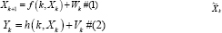
To understand the EKF, assume a non-linear dynamic system can be described by a state space model where andWk Vk found in equations 1 and 2 are white Gaussian noise process with zero mean independent covariance matrices Rk and Qk .
The function f (k, zk) is a transition matrix of a non-linear function, the matrix possibly varying over a period of time. The function h (k, Zk) is a non-linear measurement matrix also varying over time [13].
The basic idea of EKF according to [13] is linearizing the state-space model which is defined by equations 1 and 2 its current values are close to the estimated ones for each state. This update is made by function depends on the particular problem to be considered since the linear model is obtained by applying the EKF equations.
Also it is possible to say that the approximation made by the EKF occurs in two distinct phases [13]:
The first phase is the construction of the matrices in 3 and 4:
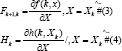
In this phase, the ijth entry Fk+l,k is identical to the partial derivative of component ith Fk, X with respect to the jth order component of X. Similarly, the ijth entry Hk is identical to the partial derivative i part of H (k, X) with respect to the jth component of X.
In the first case, the derivatives in ^Xk, are evaluated, sothat in the latter case the derivatives are evaluated at  . The entries of the matricesFk+1,k and Hk are both known as computable because and are evaluated at time k [13,16].
In the second phase of the EKF as the matrix Fk+1,k Hk are evaluated in the sequence they are used in a function of a first order Taylor series expansion to perform nonlinear functions F(k,Xk) and H(k,Xk) round  , respectively. In specific manner F (k, Xk) and H (k, xk) are estimated as follows:
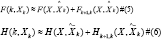
With the estimated of expressions 5 and 6 we can perform the process of approximation in the nonlinear equations 7 and 8, as shown below:

In this part, two new quantities are introduced to be calculated:

The entries in  are all known at the time k, and therefore can be considered as an observation vector at time n. Similarly, the entries in the term dk are all known at the time k[13].
Training a Neural Network with EKF
For the purposes of EKF, one MLP is used as shown in Figure 2. In this network has an input layer, a hidden layer and an output layer. The values enter to the network and the output values are connected by their weights and the mapping function.

To conduct the training of a neural network at first is necessary to organize all inputs, outputs and the network weights as state vectors [7]. Then the network computes the EKF and the same weights are used to modify the estimate predictions of filter, state vectors and observations vectors are processed.
To describe the network training, imagine a problem os estimating states where you have the following equations 11 and 12, dynamic and with the observations given [21].

The variables d and y are the desired out puts, v is the noise of random observation. Assume white gaussian noise with an average R from the covariance matrix.
Because there are a lot of articles explicity about the EKF, the algorithm will be represented in summarized form, as below:

In this way Kk+1 is the gain of the Kalman filter, Pk is the approximation error covariance matrix, and Hk+1 is the Jacobian matrix of the function with respect to the state W with current estimate  .
.
Algorithm UKF
The Unscented Transformation (UT) is a way to calculate the statistics of a random variable, which undergoes a nonlinear transformation [9].
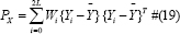
Let us consider the propagation of a variable X (n size) t hrough a nonlinear function Y=f(X). Assuming X is significant  and covariance PX . To calculate statistics Y, which forms a matrix χ; to 2L+1 vectors sigma as follows:

Where,  is the ith row or column of thematrix square root of (L+λ)Px and Wi is the weight which is associated with the ith point. The transformation procedure is as follows [9]:
First step is instantiate each point through the function to yield the set of transformed sigma points Yi = f[Xi].
In the Second step, the mean is given by the weighted average of the transformed points:

In the Third step the covariance is weights, product of the transformed points:
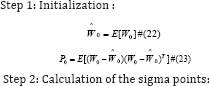
After learning the concepts of UT for applying in Kalman Filter follow these steps:
For predict a new state of system  and your associated covariance P(λ +1/λ). According Julier & Uhlmann [9] to realize this predict it is necessary to understand the effects of this noise process.
Predicting the expected observation  and the innovation covariance Pw(λ + 1/λ), this predictian should include the effects of observation noise. Finally, predict the cross-correlation matrix Pxz (λ +1/ λ) .
These steps can be easily changed by reconstructing the vectors of process and observation models of states. To do so, the state vector is augmented with the process of noise terms for a vector dimensional Lα=L+q, where:

The matrices on the leading diagonal are the covariances and off-diagonal sub-blocks are the correlations between the state errors and the process noises. Although this method requires the use of additional sigma points, it means that the effects of the process noise (in terms of its impact on the mean and covariance) are introduced with the same order of accuracy as the uncertainty in the state [9].
Training a Neural Network with UKF
The UKF algorithm for training a neural network according to Zhan & Wan [21] is very similar to EKF. In the same manner, as in EKF the weights of the connections must be in state vector format. For UKF states are calculated by the Unscented Transform (UT). Thus, it propagates by analytical form through the non-linear system without the need to measure the Jacobian matrix.
The UKF is presented below in four basic steps [21]:
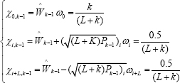
Where, i =1,2,..., L and L is the state dimension. Parameter k is used to control the covariance matrix.

Numerical Testing Results
The simulations were carried out in Matlab using Recursive Bayesian Estimation Library (REBEL) by [17] on a AMD Quadricore PC with 3.0-GHz CPU and 8 Gb memory. An Multilayer Network was used to approximate the following nonlinear function that is used for benchmark purposes.

The input and output  of the function in equation 34 are noiseless, while noisy counterparts will be used for NN training. Specifically, 100 noisy data sets were randomly generated for training with
  where k is the data set index, k ∈ [1,2,..., 100], and the noisy terms vkηk N ~(0,1). The parameters α and β are used to control the strength of the noise. The Log-sigmoid function in the hidden layer.
The test was carried out the test using various numbers of neurons (6, 8 and 10) in the hidden layer, evaluating the impact of the number of neuron in hidden layer, depending on the Mean Square Error (MSE) obtained during the training of the Neural Network.
In Table 1 the training was carried out using the following parameters α and β = 10-2 , which are responsible for the magnitude of the degree of error in input data.Note that using 6 or 10 neurons in the hidden layer the occurrence of MSE, increase during the training time.
Linear Regression (R) was evaluated against the training data and results of the neural network, denotes ensure the accuracy of the training, being used as a parameter to choose the number of neurons in the hidden layer for more effective training.
Using 8 neurons in hidden layer by means of training algorithms compare the EKF and UKF, the results are shown in Figure 3.
The aforementioned comparisons were performed in the same way that data contained in Table 2 using (6, 8 and 10) neurons in hidden layer. The value of α and β = 10-3 . Note that the pattern of errors in the Table 1 & 2 are repeated when 6 and 10 neurons are used in the hidden layer, however, the EKF filter using 6 neurons in the hidden layer is a significant improvement over the use of 8 and 10 neurons in the hidden layer.

It was decided to use 8 neurons in the hidden layer for comparing the EKF and UKF training algorithms presented in Figure 4 because accuracy is improved as demonstrated by Linear Regression parameter (R) in Table 2.

Figure 3 shows the best rate of UKF filter learning until iteration 75. In iterations 45, 63 and 75, there is a significant decrease in MSE training. The EKF filter tends to start a better learning at iteration 70. The oscillations presented in training rate are due to large non-linearity of the input data, because of the equation 34 used in the simulation.

Figure 4 shows the fastest learning UKF filter until iteration 30. From the iteration 35, the two training filters tend to have a good generalization of the function, and MSE are close until the 100 iterations. It is demonstrating a lower noise input data, helps learning rates of the training algorithm.

The minor errors were obtained by the UKF filter in iterations 45, 63 and 75, showing the best performance of the EKF filter in training Neural Networks for prediction of nonlinear systems.
Conclusion
This work demonstrates the training of a multilayered neural network (MNN) using the Kalman filter variations. Kalman filters estimate the weights of a neural network, considering the weights as a dynamic and upgradable system. The Extended Kalman Filter (EKF) is a tool that has been used by many authors for the training of Neural Networks (NN) over the years. However, this filter has some inherent drawbacks such as instability caused by initial conditions due to linearization and costly calculation of the Jacobian matrices. Therefore, the Unscented Kalman Filter variant has been demonstrated by several authors to be superior in terms of convergence, speed and accuracy when compared to the EKF. Training using this algorithm tends to become more precise compared to EKF, due to its linear transformation technique known as the Unscented Transform (UT). The results presented in this study validate the efficiency and accuracy of the Kalman filter variants reported by other authors, with superior performance in nonlinear systems when compared with traditional methods. Such approaches are still little explored in the literature.
Acknowledgement
We thank FAPESP for financial support under Grant 2015 / 23297-4.
References
- McCulloch, Warren S, Pitts W (1943) A Logical Calculus of the Ideas Immanent in Nervous Activity. The Bulletin of Mathematical Biophysics 5(4): 115-133.
- Hebb OD (1999) The Organization of Behavior: A Neuropsychological Approach. John Wiley & Sons.
- Rosenblatt F (1958) The Perceptron: A Probabilistic Model for Information Storage and Organization in the Brain. Psychological Review 65(6): 386.
- Minsky, Marvin, Seymour P (1969) Perceptrons. MIT press, USA.
- Hunt KJ, Sbarbaro S, Zbikowski R, Gawthrop PJ (1992) Neural Networks for Control Systems-A Survey. Automatica 28(6): 1083-1112.
- Hopfield, John J (1982) Neural Networks and Physical Systems with Emergent Collective Computational Abilities. Proc Nat Acad Sci 79(8): 2554-2558.
- Ronghui Z, Wan J (2006) Neural Network-Aided Adaptive Unscented Kalman Filter for Nonlinear State Estimation. Signal Processing Letters 13(7): 445-448.
- Dario B, Morgado-DF (2013) A Survey of Artificial Neural Network Training Tools. Neural Computing and Applications Springer, London, England 23(3-4): 609-615.
- Ronald WJ (1992) Training Recurrent Networks Using the Extended Kalman Filter. Neural Networks International Joint Conference 4: 241246.
- Singhal S, Lance W (1989) Advances in Neural Information Processing Systems 1. USA: Morgan Kaufmann Publishers Inc pp. 133-140.
- Puskorius, Gintaras V, Feldkamp LA (1991) Decoupled Extended Kalman Filter Training of Feed forward Layered Networks. Ijcnn-91- Seattle International Joint Conference 1: 771-777.
- Puskorius, Gintaras V, Feldkamp LA (1994) Neurocontrol of Nonlinear Dynamical Systems with Kalman Filter Trained Recurrent Networks. Neural Networks, IEEE Transactions 5(2): 279-297.
- Haykin, Simon S, Haykin SS (2002) Kalman Filtering and Neural Networks. Wiley Online Library.
- Stubberud SC, Kramer KA (2008) System Identification Using the Neural-Extended Kalman Filter for State-Estimation and Controller Modification. IEEE International Joint Conference pp. 1352-1357.
- Adnan R, Ruslan FA, Samad AM, Zain AM (2013 New Artificial Neural Network and Extended Kalman Filter Hybrid Model of Flood Prediction System. Signal Processing and Its Applications (Cspa), 9th International Colloquium pp. 252-257.
- Julier, Simon J, Uhlmann JK (1997) A New Extension of the Kalman Filter to Nonlinear Systems. Aerospace/Defense Sensing, Simul and Controls 3: 3-32.
- Wan EA, Van der Merwe R (2000) The Unscented Kalman Filter for Nonlinear Estimation. Adaptive Systems for Signal Processing 2000: 153-158.
- Gustafsson F, Hendeby G (2012) Some Relations Between Extended and Unscented Kalman Filters. Signal Processing, IEEE Transactions 60(2): 545-555.
- Trebaticky P, Pospichal J (2008) Neural Network Training with Extended Kalman Filter Using Graphics Processing Unit. Lecture Notes in Computer Science. Springer Berlin Heidelberg pp. 198-207.
- Lima DP, Kato ERR, Tsunaki RH (2014) A New Comparison of Kalman Filtering Methods for Chaotic Series. Systems, Man and Cybernetics (Smc) pp. 3531-3536.
- Iiguni Y, Sakai H, Tokumaru H (1992) A Real-Time Learning Algorithm for a Multilayered Neural Network Based on the Extended Kalman Filter. Signal Processing, IEEE Transactions 40(4): 959-966.


