


Displacement Analysis of Fault Zones Applying GNSS Technology in Vietnam
Ngoc Ha Hoang*
Hanoi University of Mining and Geology, Hanoi, Vietnam
Submission: July 22, 2021; Published: August 24, 2021
*Corresponding author: Ngoc Ha Hoang, Hanoi University of Mining and Geology, Hanoi, Vietnam
How to cite this article: Ngoc Ha H. Displacement Analysis of Fault Zones Applying GNSS Technology in Vietnam. Insights Min Sci technol.2021; 3(1): 555602. DOI: 10.19080/IMST.2021.03.555602
Abstract
In this article, a method of assessing the displacement of the fault zone has been studied on the basis of using Global Navigation Satellite System (GNSS) network measurement data in cycles and applying the theory of free mesh adjustment and S- transformation, Kalman filtering technique, and combined with the theory of variance with the error of the original data to analyze and predict the displacement in the experimental area in the south of Vietnam. The analysis concludes the shift based on the t- distribution. In the study static and dynamic models were considered and gave consistent calculation results. The theory has been proved to develop Kalman filter technique for deformation analysis and prediction problem applying GNSS technology. The main result in this paper is to apply the theory of free network adjustment and Kalman filter to determine the displacement parameters of the fault zone based on the GNSS measurement data of 3 measuring cycles. This result allows to expand the scope of application of GNSS technology for monitoring and analysis of landslides; subsidence and displacement of the Earth’s crust on a local scale as well as a territorial extent in Vietnam and can use data from GNSS CORS observation stations.
Keywords: Satellite; Geodynamics; S- transformation; Earth’s crust; Geodetic network
Introduction
The application of Global Navigation Satellite System (GNSS) technology has created a very effective breakthrough in geodynamics and deformation monitoring. GNSS networks are three-dimensional spatial networks, so iterative measurement allows simultaneous determination of both horizontal and vertical displacement vectors of the earth’s crust. With the basic advantages of satellite positioning technology such as not requiring navigation between points, measurements can be carried out in all weather conditions, it is possible to quickly develop a geodynamic network on a large scale. territory. A number of studies have mentioned the problem of applying GNSS technology to study geodynamics [1-4]. On the application of Kalman filter, have focused on building models applying Kalman filter to analyze geodetic monitoring observations [5], applied Kalman filter with color noise to study deformation analysis [6].
In Vietnam, the dynamic geodetic network is built according to modern and solid standards for long-term use. The location of the landmark on the bedrock has been surveyed and constructed by surveying experts and tectonic geologists. The design of the landmark structure has referenced the landmark systems of the US and Europe. Repeated measurements of the GNSS geodynamic network have been performed over areas of the active fault zone with a once a year measurement period, starting from 2013 to 2015. In Vietnam, satellite positioning technology has been applied in a number of studies on the displacement of the earth’s crust such as the study of the displacement of the Da River fault zone and the Son La - Bim Son fault zone [5]. Applied the GPS free network adjustment theory in analyzing the displacement of the Saigon River fault [7].
In this paper, we present the results of applying the S- transformation combined with the Kalman filter technique to analyze and predict the displacement on the experimental area of the 7-point GNSS network in the southern region.
Methodology
Baseline GNSS free network adjustment and S- transformation
Suppose in the GNSS network there are m points to be determined. The unknowns will be the geocentric coordinates which will be (Xi, Yi, Zi), (i=1, 2...m). The system of equations of corrections for n baselines has the following form:
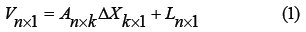
Here A is the coefficient matrix with the coefficients +1 and -1 corresponding to the coordinate components in the baseline measurement (ΔXij, ΔYij, ΔZij). Where i and j are the number of GNSS points.
ΔXk×1 is the vector of unknowns, Vn×1 is vector of corrected numbers
k=3 x m
The weight matrix P has the form:
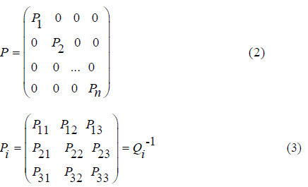
Qi - the covariance matrix of the i -th baseline measurements The normal system of equations has the form:
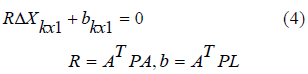
We have the condition that the constraint has the following form:
CΔX = 0 (5)
The unknown vector is calculated according to the formula:
ΔX = −R ~ b (6)
In which, R~ is the general inverse matrix:
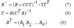
For a baseline GNSS network (ΔX, ΔY, ΔZ), the matrix B has the form:
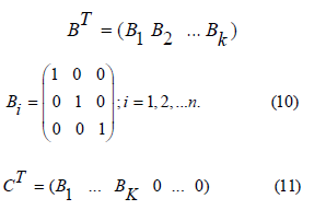
In the case of G = B, the general inverse matrix is calculated by the formula:
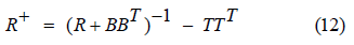
Here the matrix T is defined by the formula (8)
For an accurate assessment, the following quantities need to be calculated:
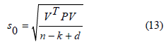
Where:
n is the number of measurements
k - number of unknowns
d is the number of defects of the network (d = 3).
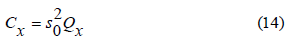
The covariance matrix is determined according to the following formula:
S- transformation
In each cycle, the GNSS network is adjusted according to formulas (1) to (14). As a result, the coordinate vector x of the points and the covariance matrix Cx have been calculated. For deformation analysis, the data need to be performed on a reference system. The data of geodetic networks measured and calculated in different periods are fed into a positioning system by the S-transformation.
The S transformation is performed using the following formulas (1), (11):
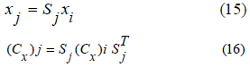
Here xj and xi are coordinate vectors of the network points at j and k positioning coordinate systems
(Cx)j, (Cx)i are covariance matrices at the j and i positioning coordinate systems.
The matrix Sj is defined as:
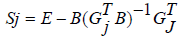
Here the matrix Gj is determined by the formula (11) for positioning coordinate system j
E- Unit matrix.
Application of the kalman filter
The kinematic model over time with coordinates, velocity and acceleration is represented by the following formula:
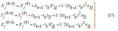
where Xj(k+1), Yj(k+1), Zj(k+1): coordinate of point j at time (tk+1) period.
Xj(k), Yj(k), Zj(k): coordinate of point j at time (tk) period.
vxj, vyj, vzj: velocities of X, Y, Z coordinates of point j
axj, ayj, azj: accelerations of X, Y, Z coordinates of point j
k=1, 2, . . ., I (i: measurement period number)
j=1, 2, . . ., k (k: number of points)
The system of equations of the motion model used to predict motion parameters by Kalman filtering technique in 3D meshes can be represented as a matrix as follows:
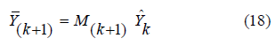
Where:
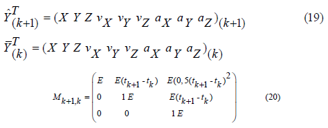
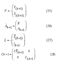
where ȲT(k+1): prediction status (position, velocity, acceleration) vector at period (k+1)
ŶTk: state vector at period k
The equation with the noise factor will be as follows:
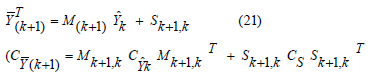
CŶk: the covariance matrix of state vector at period k.
CS: the covariance matrix of system noises at period k.
At time tk+1, we measure the GNSS network and can establish a system of measurement equations (filter equations) as follows:
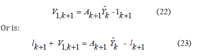
Combining expressions (18) and (23) we have the following formula:
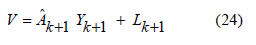
Here we denote:
The Ak+1 matrix in expression (26) in the case of taking the measured value l equal to the value corrected after the network adjustment at period (k+1) will be:
Here: E(kxk) - Unit matrix, k- number of unknowns.
Applying the theory of variance with the original data information and the recurrence formula in calculating the covariance matrix of state vectors
System of equations (24) is the system of equations of the corrected numbers in the least squares method. The system of normal equations will be:
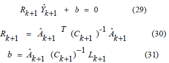
According to Kalman filter theory, the Gain matrix will be:

The state vector at time tk+1 will be:
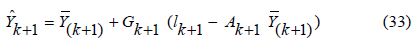
From expressions (26), (28) and (30) we have:

The covariance matrix of the state vector Ŷk+1 will be:
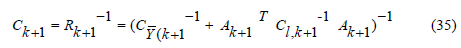
Following the recurrence formula (8), we have the expression:

Here the matrix:
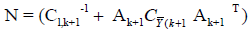
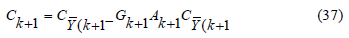
Combining the expressions (32), (35), (36) we have the covariance matrix of the state vector at time tk+1 which will be:
Numerical Application
Introduction to experimental data
To study the shifting activities of the southern region of Vietnam, a monitoring network has been established including 7 points, measured by GNSS technology. The landmark is built according to the standard of mandatory centering landmarks placed on the bedrock. In Figure 1, the location of the monitoring landmarks of the study area is shifting. Repeat measurement for 3 cycles 2013, 2014, 2015, time interval between cycles is one year.

Calculation results and discussion
Static model analysis
In the first step, applying the 3D free network adjustment to process the Baselines, the network coordinates were obtained in the 2013 2014 and 2015 cycles. Conduct assessment of the change of milestones between 2 cycles: TX=dX/md\x, TY=dX/md\Z , TZ=dZ/ md\Z. Check the Criteria (t-distribution) [8]: ǀTX ǀ< qX, ǀ TY ǀ< qY, ǀ TZǀ< qZ,. If the test value is greater then the critical value, then there are significant deformations in the points [9-14].
The evaluation results show that score 1 is stable. The remaining points move. Performing the transformation S, presented in section 5.2.1 using the positioning point as point 1, we have the matrix S as follows:
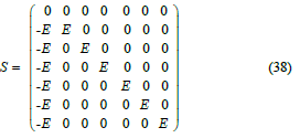
Here the block matrices: E(3x3)- unit matrix; 0(3x3)- matrix all zeros.
Performing the S transformation presented in section 5.2.1, we have the results of calculating the displacement data of period 2 and period 3 compared with period 1 (in mm) and diagonal components of the matrix. covariance. These results are presented in Tables 1 & 2. Assessing the shift of landmarks between 2 cycles according to the criteria ǀTX ǀ< qX, ǀ TY ǀ< qY, ǀ TZǀ< qZ, we see a shift of points from 2 to 7.


Analysis of motion according to kalman filter
In the Kinematic Model we have not only specifying the coordinate displacement parameters of the points (dX, dY, dZ), but also displacement parameters such as velocity and displacement acceleration. If the parameters change significantly according to the criterion T (t-distribution), they are marked (+), not marked (-) (Table 3) [15].

Conclusion
>The proposed methodology allows displacement analysis with static and dynamic models of the Fault Zone on the basis of using GNSS data and Kalman filtering method. Both models give similar results in determining the displacement of the GNSS network. In the application of the filter Kalman has studied and theoretically proved that the covariance matrix of the state vector can be determined based on the principle of variance with the original data error of the least squares method. The proposed methodology allows to determine the displacement and acceleration of each point. These research results can be applied to geodynamic research in geology, research to identify faults and landslides, and can predict displacement with high accuracy if there are many monitoring cycles. With the use of GNSS monitoring technology that can be deployed throughout the territory and combined with the growing network of CORS stations (in Vietnam, there are currently 65 stations), opening up the possibility of monitoring and analyzing epidemics convenient timed continuous transfer with high accuracy. The proposed methodology can contribute to solving the problem of environmental impact assessment in coal exploration and mining in Vietnam [16,17].
References
- Acar M, Özlüdemir M, Çelik R, Erol S, Ayan T (2004) Landslide Monitoring Through Kalman Filtering: A Case Study in Gurpinar. XXth Congress, Istanbul, Turkey, 7: 682-685.
- Casula G (2016) Geodynamics of the Calabrian Arc area (Italy) inferred from a dense GNSS network observations. Geodesy Geodyn 7(1).
- Erol S, Erol B, Ayan T (2005) An Investigation on Deformation Measurements of Engineering Structures with GPS and Leveling Data: Case Study. In: Proceedings of International Symposium on Geodetic Deformation Monitoring: From Geophysical to Engineering Roles, Jaen, Spain, pp. 244-253.
- Shults R, Anenkov A (2018) Investigation of the different weight models in Kalman filter: A case study of GNSS monitoring results. Geodesy and Geodinamics 9(3): 220-228.
- Welsch W, Heunecke O (2001) Models and terminology for the analysis of geodetic monitoring observations. In: Proceedings of the 10th International Symposium on Deformation Measurements, Orange, California, USA pp. 390-412.
- Markuze YI, Hoang H (1991) Adjustment of Terrestrial and Satellite Space Networks. Nhedra Moscow Publishing House (in Russian), pp. 274.
- Hoang H, Pham T (2016) The application of spatial network free variance theory in analyzing the displacement of the Saigon River fault. Resources and environment (in Vietnamese) 23(253): 1-12.
- Ghilani CD, Wolf P (2017) Adjustment Computations. In: John Wiley & Sons, 6th
- Herring T, Gu C, Toksöz M, Parol J, Al Enezi A, et al. (2018) GPS Measured Response of a Tall Building due to a Distant Mw 7.3 Earthquake. Seismological Research Letters 90(1): 149-159.
- Hoang H, Truong H (2000) Basis of Mathematical Processing for Geodetic Data. Transport Publishing House (in Vietnamese).
- Hoang H (2006) Adjustment of Geodetic and GPS networks, Science and Technology Publishing House, Hanoi (in Vietnamese).
- Hoang H (2020) Modernization of Height System in Vietnam Using GNSS and Geoid Model. In: Tien Bui D, Tran HT, Bui XN. (eds) Proceedings of the International Conference on Innovations for Sustainable and Responsible Mining. Lecture Notes in Civil Engineering, Springer, Cham 108.
- Kalman RE (1960) A new approach to linear filtering and prediction problems. J Basic Eng 82(1): 35-45.
- Kotsakis C, Sideris MG (1999) On the adjustment of Combined GPS/Levelling/Geoid Networks. Journal of Geodesy 73(8): 412-421.
- Kuhlmann H, Kalman (2003) Filtering with coloured measurement noise for deformation analysis. In: Proceedings of 11th FIG Symposium on Deformation Measurements, Santorini, Greece, pp. 455-462.
- Leick A (1995) GPS Satellite Surveying. 2nd A Wiley interrscience publication John.
- Poyraz F, Gülal E (2007) Integration of theoretical and the empirical deformations by Kalman filtering in the North Anatolia Fault Zone. Nat Hazards Earth Syst Sci 7: 683-693.


