


An Efficient Breast Cancer Detection Using Jelly Electrophorus Optimization Based Deep 3D Convolution Neural Networks (CNN)
Sagarkumar Patel1* and Rachna Patel2
1 LabCorp Drug Development Inc, M.S. in Information System Security, USA.
2 Catalyst Clinical Research Llc, M.S. in Computer Science, USA
Submission: September 14, 2023; Published: September 22, 2023
*Corresponding Address: Sagarkumar Patel, LabCorp Drug Development Inc, M.S. in Information System Security, USA Cancer Ther
How to cite this article: Sagarkumar P, Rachna P. An Efficient Breast Cancer Detection Using Jelly Electrophorus Optimization Based Deep 3D Convolution Neural Networks (CNN). Canc Therapy & Oncol Int J. 2023; 25(2): 556156. DOI:10.19080/CTOIJ.2023.25.556156
Abstract
Breast cancer is one of the world’s most serious diseases that affect millions of women every year, and the number of people affected is increasing. The only practical way to lessen the impact of a disease is through early detection. Researchers have developed a variety of methods for identifying breast cancer, and using histopathology images as a tool has been quite successful. As an enhancement, this research develops a jelly electrophorus optimization-based 3D density connected deep Convolution Neural Networks (CNN) for the identification of breast cancer using histopathology images and input is collected and pre-processing is performed for improve the histopathology image’s properties.
Then the feature extraction is performed through VGG-16, AlexNet, ResNet-101, statistical features. Finally, these concatenated features are fed forwarded to 3D density connected 3D deep Convolution Neural Networks (CNN) classifier it automatically detects breast cancer effectively with the help of jelly electrophorus optimization. The proposed jelly electrophorus optimization adjusts the classifier’s weights and bias. In terms of accuracy, sensitivity, and specificity, the proposed JEO-3D deep Convolution Neural Networks (CNN) approach attains values of 93.73%, 95.31%, and 94.14% for dataset 1 and 88.75%, 90.32%, and 89.15% for dataset 2, which is more successful.
Keywords: Breast cancer detection; Jelly electrophorus optimization; 3D deep Convolution Neural Networks (CNN); VGG-16 and ResNet-101
Introduction
Breast cancer is a widespread and significant health problem that affects men and, to a lesser extent, women worldwide. It is a malignant tumor that arises from cells of the breast tissue. The World Health Organization (WHO) estimates that in 2020, it will account for around 11.7% of all new cancer cases [1]. Breast cancer incidence varies among areas and nations, with greater rates seen in developed countries [2]. The incidence of breast cancer and the high mortality rates that go along with it have a significant influence on public health [3]. Patients’ emotional, psychological, and social health is also impacted in addition to their physical health. Due to the disease’s high medical needs and prolonged treatment, healthcare systems are placed under a heavy financial load. The prevalence of breast cancer has steadily increased over time in every country. 2.3 million new instances |of breast cancer are anticipated to be diagnosed globally in 2020 [4]. Age raises the likelihood of getting breast cancer, with women over 50 accounting for the majority of cases [5-7]. Early breast cancer detection considerably improves the effectiveness of treatment and raises the likelihood of a full recovery [8]. It makes it possible for less aggressive and more focused forms of treatment, possibly lowering the need for expensive operations or chemotherapy [9]. Early diagnosis can also improve patients’ quality of life and minimize healthcare expenses related to advanced-stage therapies.
Histopathology images are critical for breast cancer identification because they give significant details about the microscopic characteristics and structure of breast tissue [10]. The existence of cancer cells, their subtypes, and the tumor grade are all determined by pathologists by examining these tissue samples taken from biopsies [11]. The cellular and tissue-level changes brought on by breast cancer can be seen by pathologists using histopathology imaging [12]. They are able to spot atypical cellular development, abnormal cell proliferation, and architectural disarray indicative of malignant development [13,14]. The diagnosis of breast cancer must include histological grading since it tells doctors how aggressive the tumor is. To define the tumor grade, pathologists employ histopathology images to evaluate the cellular properties, growth patterns, and differentiation of cancer cells [15].
Typically, breast cancers are ranked from 1 to 3, with higher rankings denoting tumors that are more aggressive [16]. Histopathology imaging is also used to assess lymph node samples obtained through a dissection of an axillary lymph node or a sentinel lymph node biopsy [17,18]. Pathologists evaluate if cancer cells have progressed to the adjacent lymph nodes in order to establish the disease’s stage and formulate a treatment strategy [19,20]. Breast cancer tissue samples histological characteristics can reveal important details about the patient’s prognosis [21]. The risk of recurrence of the disease and patient survival rates can be predicted using the tumor grade, the degree of lymph node involvement, and other histological features.
Artificial neural networks with numerous layers are trained in the deep learning field of machine learning and artificial intelligence to automatically recognize hierarchical data representations. Because they are designed to mimic the structure and operation of the human brain, these neural networks can learn sophisticated patterns and relationships from massive amounts of data [22]. Deep learning has become an effective technique for tackling many different issues, particularly in image analysis and computer vision duties [23]. Deep learning has made significant progress and shown great potential in the field of medical imaging. Medical image analysis has historically depended on manually created features and domain-specific algorithms, which frequently needed specialized knowledge and had a limited capacity to recognize detailed patterns in complicated images [24,25]. Deep learning techniques, particularly CNN, have significantly improved the accuracy and effectiveness of medical image analysis, particularly histopathological image interpretation [26]. There have been considerable improvements in diagnosis, treatment planning, and patient care as a result of CNN extraordinary performance in classifying medical images, particularly histopathological images [27,28]. These deep learning-based methods are propelling further advancements in medical imaging and opening the door for more precise, effective, and individualized healthcare solutions.
The main aim of the research is to detect breast cancer using jelly electrophorus optimization-based 3D density connected deep convolution neural networks (CNN). Input is collected and pre-processing is performed for improve the histopathology image’s properties. Then the feature extraction is performed through VGG-16, AlexNet, ResNet-101, statistical features. These features are concatenated using multiplied features patterns so it retains the unique characteristics of each feature, potentially leading to better model performance. Finally, these concatenated features are fed forwarded to 3D density connected 3D deep CNN classifier it will automatically detect breast cancer effectively with the help of jelly electrophorus optimization. The contributions of the research are,
Jelly Electrophorus Optimization (JEO)
The proposed jelly electrophorus optimization is developed by the standard hybridization of jelly and electric fish algorithm. In electric fish algorithm the escaping capability from predators is not interpreted so it faced difficulties in handling largescale optimization problems and slower convergence rates. To improve convergence rate and performance the jellyfish time control mechanism is merged with electric fish, so it generates nematocysts to capture prey and defend themselves from potential threats.
JEO-3D Density Connected Deep Convolution Neural Networks (CNN)
3D Deep CNN is a convolutional neural network designed to process and analyze three-dimensional data. It extends the concept of standard two-dimensional convolution neural networks (CNN) s to three-dimensional space, allowing the network to capture spatial patterns and temporal dynamics in the data. The proposed 3D deep CNN optimization increases detection speed while improving the classifier’s intrinsic properties. The optimization’s stability factor helps to reduce misclassification, while internal factors such as weights and bias are optimized to reduce detection time.
The following is a description of the manuscript’s flow: Section 2 lists the reviews breast cancer detection. In section 3, the suggested jelly electrophorus optimization-based 3D density connected deep CNN is described along with its method, operation, and mathematical model. In section 5, the results are described in detail. Section 5 concludes the research.
Literature review
The reviews of the breast cancer detection are as follows [1] presented an innovative transfer learning-based technique to automate the classification of breast cancer from histopathology images. Their approach successfully amalgamates binary and eightclass categories, accounting for both magnification-dependent and magnification-independent factors. This method sped up training while preventing over-fitting, but it had a flaw. Breast cancer histopathology image identification was demonstrated by [13] using a hybrid convolution and recurrent deep neural network technique. Intricate patterns and features in the input data could be captured by this method’s learnt sophisticated and hierarchical representations of data, but its computational complexity was higher [8] introduced a customized residual neural network-based approach to identify breast cancer using histopathology images. While this method exhibited promising performance across various magnification factors, it did encounter challenges related to overfitting and vanishing gradient issues. An automated method for diagnosing breast cancer tumors using histopathological pictures was introduced by [5].
Although it used more memory, this approach allowed for a smoother gradient flow during back propagation [1] devised enhanced techniques for different CAD phases with the aim of reducing the variability gap among observers. Their approach significantly improved breast cancer classification accuracy by tackling the challenge of low-density areas and leveraging the cluster assumptions feature to select appropriate prospective samples. Meanwhile [22] introduced a patch-based deep learning approach utilizing the Deep Belief Network to effectively detect and classify breast cancer in histopathology images. The overfitting problem was addressed by this method’s automatic learning of the best features, but its scalability and interpretability were constrained.
Phylogenetic diversity indices are used by [24] to define images and create a model for categorizing histological breast images into four classes. Accuracy and larger dimensional feature spaces were reached by this method, however hyperparameter tweaking was challenging. Breast tumor type assessment was addressed by [29] by processing histopathology images that were obtained from the lab. Particularly on complex and heterogeneous datasets, this strategy outperformed individual weak learners in terms of accuracy, although it had an overfitting problem.
Challenges
The difficulties encountered during the research are listed as follows.
i. Annotated 3D mammograms and breast MRI scans might be difficult to get in large and varied datasets. Additionally, the dataset may be class imbalanced, with more benign cases than malignant cases, which makes it more difficult for the model to draw lessons from the minority class.
ii. Image quality, resolution, and noise might vary depending on the imaging techniques and data sources used in medical imaging. It is difficult to create models that can handle this variety.
iii. While deep 3D convolution neural networks (CNN)s can make precise predictions, they might not go into great depth to explain their choices. Understanding the model’s reasoning is essential in medical applications to promote trust and support expert judgment.
iv. When resources are limited, 3D convolution neural networks (CNN)s might be more difficult to deploy since they frequently demand a lot of memory to store the model parameters and intermediate data during training.
v. High sensitivity and specificity are needed to identify early-stage breast cancer or minor mammography abnormalities, which can be difficult for the model to accomplish.
Proposed methodology for breast cancer detection
The goal of the research is to identify breast cancer using a deep CNN classifier based on jelly Electrophorus optimization. The initial collection of input histology images from the repository is followed by image preprocessing to improve the histopathology image’s properties. After pre-processing, feature extraction is performed using VGG-16, AlexNet, ResNet-101, statistical features. These features are concatenated using multiplied features patterns so it retains the unique characteristics of each feature, potentially leading to better model performance. Finally, a 3D density connected 3D CNN classifier is fed these extracted features in order to detect breast cancer. The jelly Electrophorus optimization was created by combining the qualities of jelly fish optimization [30] and electric fish optimization [31]. This hybrid optimization effectively tunes the classifier’s internal attributes, which speeds it up. The proposed breast cancer method’s systematic approach is shown in Figure 1.
Input
Histopathology images, which are used as an input, are microscopic images of tissue samples acquired from patients. Here, the input information for identifying and categorizing breast cancer is taken from a Breast Cancer Histopathological Image Classification (BreakHis) and breast cancer histopathological annotation and diagnosis (BreCaHAD) database and expressed mathematically by,
Here, H stands for the data that was gathered, p is the number of various data sets, and i is the many data attributes.
Pre-processing
During the preprocessing stage, the breast biopsy procedure is done to locate the tumor, lumpy area, or aberrant region. To make a diagnosis, the pathologists take a tissue sample from the affected area. A trio of techniques, comprising surgical biopsy, core needle biopsy, and surgical biopsy, offer the means to detect diseases within the tissues. Subsequently, the pathology department analyzes both the patient’s specifics and tissue characteristics to determine the most suitable disease category.
Where, the pre-processed data is denoted as H*i

Feature extraction
Feature extraction is the process of identifying and measuring relevant qualities or patterns from images to reflect tissue architecture, cell nuclei, or specific pathogenic defects in histopathology image analysis. After that, these characteristics are used for additional analysis, classification, or diagnosis. Histopathology images, which are obtained from tissue samples stained to emphasize particular components, are essential for pathological diagnostics and medical research. An approach that is frequently employed in image analysis and pattern recognition tasks, particularly for texture analysis, is feature extraction employing statistical and multivariate texture pattern features. To create the texture patterns used in the method, descriptive statistical features that describe image portions or patches are extracted and combined with the image data.
VGG-16
The deep CNN VGG-16 is capable of learning hierarchical features from images. These features can be used to depict different patterns and structures seen in tissue samples in the context of histopathology images. VGG-16 has 16 layers, comprising 3 fully linked layers and 13 convolutional layers. It requires a 224x224 pixel input image. Resizing the image to 224x224 pixels is a normal preparation step for VGG-16. Changing the image’s color space from RGB to BGR and subtracting from each channel the average pixel intensity from the ImageNet dataset. The VGG-16’s fully connected layers are unique to picture categorization. Remove these fully connected layers to keep only the convolutional layers since we are using VGG-16 to extract features.
The output from one of the convolutional layers can be obtained by running the preprocessed histopathological image through the modified VGG-16 network. The high-level patterns and structures visible in the histopathological image are represented by these output features. Due to its deep architecture, it can recognize intricate hierarchical patterns and features in images. Edges, textures, and colors are examples of low-level features that can be extracted using VGG-16 in a generic way. Even though there is a lack of specific training data, these general features can be helpful for a variety of computer vision applications, such as histopathology image interpretation.
ResNet-101
The ResNet architecture, also known as the Residual Network, has a variation called ResNet-101. It is a deep CNN that is renowned for its capacity to circumvent the vanishing gradient issue, which facilitates the training of extremely deep networks. Among other computer vision tasks, the 101-layer ResNet-101 network is often used for feature extraction in histopathology image processing. Remaining blocks are a concept that is introduced in ResNet-101. These blocks enable the gradient to flow directly across the network by skipping one or more layers via shortcut connections (also known as skip connections).
This architecture makes it simpler to train extremely deep networks, which was difficult with earlier designs. The photos should be normalized to have pixel values within a certain range and resized to the input size requested by ResNet-101. Similar to VGG-16, ResNet-101’s fully connected layers that are specific to image classification tasks should be removed when utilizing it for feature extraction. This makes certain that only the convolutional layers that capture important characteristics are kept. Run the previously processed histopathological image through the updated ResNet-101 network to obtain the output from one of the convolutional layers. High-level feature representations of the input image will be included in the output. By letting the network concentrate on learning the residual features rather than attempting to learn the complete mapping directly, the residual blocks in ResNet-101 enable superior feature learning. As a result, significant features are learned more effectively, and the portrayal of intricate patterns and structures in histopathological images may improve.
AlexNet
AlexNet is an eight-layer deep CNN with five convolutional layers and three fully linked layers. Its purpose was to process 227x227 pixel images. The photos should be normalized to have pixel values within a certain range and shrunk to the input size required by AlexNet, which is typically 227x227 pixels. Remove the fully connected layers from the model when using AlexNet for feature extraction because they are designed for image classification tasks alone. This makes certain that only the convolutional layers that capture important characteristics are kept. Run the previously processed histopathological image through the altered AlexNet network to obtain the output from one of the convolutional layers. High-level feature representations of the input image will be included in the output. architecturee readily prototyped and tested in many computer vision tasks because it is very simple in comparison to more modern architectures. This can be helpful for initial research or as a jumping-off point before delving at more complicated architectures.
Statistical features
The distribution and shape of the pixel intensities inside the image can be learned from statistical features, which are frequently employed to characterize and analyze histopathological images.
i. Mean: The image’s mean pixel intensity value is represented by the mean. It is determined by adding up all of the pixel intensities and then subtracting the total number of pixels. The average gives a general assessment of the image’s brightness.
ii. Variance: The variation of an image’s pixel intensity levels is a measure of their spread or dispersion. The amount of deviation from the mean in the pixel intensities is measured. A larger range of pixel intensities is indicated by higher variance, whereas a more uniform distribution is implied by lower variance.
iii. Standard Deviation: The square root of the variance is used to determine the standard deviation. It provides a gauge for the degree of variance or uncertainty in the values of pixel intensity. More variation in pixel intensities is indicated by a higher standard deviation.
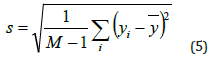
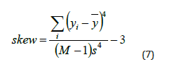
iv. Skewness: The asymmetry of the pixel intensity distribution is measured by skewness. In comparison to a normal distribution, it shows whether the distribution is skewed to the left or to the right. A symmetric distribution is suggested by a zero-skewness value.

v. Entropy: Entropy is a metric for the randomness or ambiguity of the distribution of pixel intensities in an image. The amount of data needed to describe the distribution is quantified. More complex and unpredictable patterns of pixel intensities are implied by higher entropy.
vi. Kurtosis: Kurtosis describes the pixel intensity distribution’s form, particularly the existence of strong tails or outliers. When compared to a normal distribution, positive kurtosis implies a more peaked distribution with heavier tails while negative kurtosis indicates a flatter distribution with lighter tails.
Multiplied feature patterns: Multiplied feature patterns concatenated the ResNet, AlexNet, VGG-16, statistical features and the final output are generated as a one-dimensional feature vector of dimension [n× 28 × 28 ×8]. By combining features through concatenation and leveraging the average outputs of pre-trained models, the proposed approach demonstrates its efficacy in event detection, leading to enhanced prediction accuracy. Concatenated features enable feature fusion, allowing the learning algorithm to exploit the complementary nature of different features, leading to a more powerful and informative representation. The mathematical equation becomes,
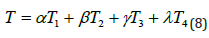
Where, T1 denotes VGG-16 features, T2 denotes ResNet-101 features, T3 denotes the AlexNet features and T4 denotes statistical features. Here α ,β ,γ ,λ relies in [0, 1] and α + β +γ +λ Figure 2

3D Density connected 3D deep convolution neural networks (CNN): 3D medical images are a type of volumetric data that 3D CNN is made to handle. The model can record spatial interactions along all three dimensions by utilizing 3D convolutions, which is vital for applications where proper feature extraction and analysis depend on 3D context. The network’s first layer is made up of 3D convolutional layers that use 3D filters to extract spatial characteristics from the volumes of 3D images. To identify regional trends and features, the filters move over the volumes’ width, height, and depth. Dense connections enable information to move from one layer to another more directly, potentially resolving the vanishing gradient issue and encouraging feature reuse. The model then conducts classification operations using the retrieved features after feeding them into fully linked layers. For the purpose of detecting breast cancer, the output layer might be created to categorize the input volume as benign or malignant. The model is trained using data volumes that have labels indicating whether they are malignant or benign. The model’s parameters are modified using jelly Electrophorus optimization during training to lower the classification error Figure 3.

3D convolution: When employing 2D convolution within a preceding layer’s feature map surroundings, a 2D CNN convolutional layer arranges its units in planes that share the same set of weights. These units possess receptive fields of a size equivalent to the 2D convolution kernel. The convolution layer combines the outputs from each plane to generate a feature map. On the other hand, a 3D CNN utilizes a 3D kernel to convolve over a stack of consecutive frames, resulting in 3D convolution. The output of this 3D convolution on a cube becomes another cube, allowing 3D CNN to capture both spatial and temporal structures. In contrast, 2D CNNs focus solely on spatial information during convolution and do not account for temporal aspects. Formally, the value in the jth cube of the ith layer at point (u,v,w) is given by,

Where, Xi , Yi , and Zi represent the kernel’s height, breadth, and length, respectively. The number of cubes in the index of the
preceding layer is n . The kernel’s (x, y, z)th link to the previous
layer’s sth cube is known as  . The location output from the jth cube in the ith layer is denoted by the symbol
  and aij is the bias. The activation function denoted by the variable f ( ) is a sigmoid function, tan hyperbolic function, or rectified linear
unit (RELU).
and aij is the bias. The activation function denoted by the variable f ( ) is a sigmoid function, tan hyperbolic function, or rectified linear
unit (RELU).
3D CNN architecture: Within the network, there exists a sole input layer, accompanied by three 3D convolutional layers, two pooling layers, two fully connected layers, and an H -way fully connected layer that employs a SoftMax function for its final stages. Here, H denotes the total number of motions targeted for recognition. The input layer, positioned at the top, defines the input’s size, taking the form of a cube with dimensions of 1× he ×we × c . Here, f represents the number of channels, while he and we indicate the height and breadth of each individual image.
The 3D kernel size is aptly described as t × s × s , where t pertains to temporal depth, and s refers to the spatial dimension. In the setup, the three convolutional layers encompassed 32, 64, and 64 kernels, with each kernel measuring 3 × 3 × 3 in size. The stride for convolution remained fixed at 1 × 1 × 1. Following a pooling layer with dimensions s × 1 × 1, both the second and third convolutional layers were subjected to zero padding with dimensions of 0 × 1 × 1, thereby restricting sub-sampling to the temporal domain. In the two fully connected layers, there were a total of 512 and 128 neurons, respectively. Throughout, the RELU technique was utilized to activate all hidden layers.
Proposed jelly Electrophorus optimization
The proposed jelly electrophorus optimization is developed by the standard hybridization of jelly and electric fish algorithm. In electric fish algorithm the escaping capability from predators is not interpreted so it faced difficulties in handling largescale optimization problems and slower convergence rates. To improve convergence rate and performance the jellyfish time control mechanism is merged with electric fish, so it generates nematocysts to capture prey and defend themselves from potential threats.
Motivation: One of the newest swarm-based metaheuristics is called the Jellyfish Search optimizer. The JS algorithm imitates jellyfish in the ocean as they search for food. Jellyfish in the ocean move in two primary ways: (1) following ocean currents to produce jellyfish swarms, also known as jellyfish blooms; and (2) moving within jellyfish swarms. Both the diversification and the intensity of the search are taken into account by the JS optimizer. In fact, jellyfish initially follow the currents of the water in search of food sources. As the swarms of jellyfish become larger over time, jellyfish often alternate between passive and active motions.
The transition between these two forms of motion is controlled by a temporal control system. Electrocytes, a specific type of cell that resembles a disc and is utilized to create an electric field, are found in the electric organ of electric fish. This organ is typically found at the back of the body. The simultaneous excitation of electrocytes is referred to in the literature as a electric organ discharge. EOD’s frequency and amplitude are its distinguishing features. The EOD frequency and the interval that separates successive electric pulses are inversely connected. Both the novelty factor (rapid increase) and the stimulus distance (regular increase) have a significant impact on it. The EOD amplitude, however, is related to the size of the fish and degrades with the inverse cube of its distance from the body surface because of the electrocytes that are produced during growth.
Mathematical model of the proposed jelly Electrophorus optimization:
In the subsequent section, we delve into the mathematical model governing the behavior of the novel jelly electrophorus optimization technique.
i. Population initialization
The search space’s borders are used while determining the initial dispersion of the electric fish population ( S )
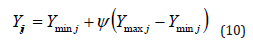
Where, the two-dimensional search space Yij denotes the location of the ith person in the population of size |S| (i =1,2,....|S| ). The lower and upper limits of dimension j | j∈1,2,.....de are designated as Ymin j and Ymax j , respectively. The value ψ ∈[0,1] is chosen at random from a uniform distribution. Following the start phase, individuals of the population use their active or passive electro location ability to move about the search space. The frequency is a key component in the EFO algorithm that optimizes exploration and exploitation and affects whether a person would engage in active or passive electro location. It forces better people (active mode people), who are more likely to live nearby promising regions, to take advantage of their surroundings and it encourages other people (passive mode people), to search the space and find new regions, which is crucial for multimodal functions.
ii. Fitness evaluation: In this technique, like in nature,
those with a higher frequency employ active electro location
whereas others use passive electro location. The frequency value
of a particular person lies between the minimum value, Fmin ,
and the maximum value, Fmax . The fitness value of an individual
determines its frequency value  because an electric fish’s frequency value at a given time s is entirely associated with its
proximity to a food source,
because an electric fish’s frequency value at a given time s is entirely associated with its
proximity to a food source,
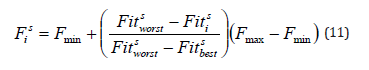
Where  represents the fitness value of the ith person at iteration s,
  represents the worst and
  represents the best fitness values, obtained from members of the current population at iteration s , respectively. When calculating
probability, the frequency value is used. Fmin and Fmax are set
to 0 and 1, respectively.
represents the best fitness values, obtained from members of the current population at iteration s , respectively. When calculating
probability, the frequency value is used. Fmin and Fmax are set
to 0 and 1, respectively.
iii. Calculate amplitude: Electric fish have knowledge about both amplitude and frequency. A fish’s active range when actively electro locating and the probability that it will be seen by other fish passively electro locating are determined by the strength of the electric field decaying with the inverse cube of distance. An individual’s amplitude depends on the importance of their prior amplitudes ( β in equation 12), therefore it is possible that it may not vary much over time. The ith individual’s ( Bi ) amplitude value is determined as follows,
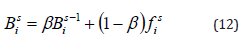
Where, β | β ∈[0,1] stands for a constant value that determines the magnitude of the previous amplitude value. The starting frequency value fi is set to the ith individual’s initial amplitude value in EFO. A fish’s (or an individual’s) frequency and amplitude parameter values are changed in accordance with how close they are to the best source of prey. Every time the algorithm iterates, the population is divided into two groups based on each person’s frequency value those doing active electro location (SA) and those conducting passive electro location (SP). Because an individual’s frequency is compared to a uniformly distributed random value, the higher the frequency value a person has, the more likely it is to undertake active electro localization. The search is then carried out simultaneously by individual in SA and SP.
iv. Local searching: Fish only have a biologically efficient range of active electro location that is about half their size, and this is where they can detect prey. Outside of this range, fish are unable to detect prey. Fish are therefore able to discover any nearby food source because to this skill. These active electro location features serve as the foundation for the algorithm’s local search or exploitation capabilities. In electric fish, all active mode individuals travel throughout the search space by changing their features. Active mode individuals execute active electro locating. To prevent people from straying too far from the promising area, only one randomly selected parameter is permitted to be changed.
Depending on whether neighbors are present within its active range, the ith individual’s movement may change. It walks randomly around its range if there are no neighbors; otherwise, it randomly selects one neighbor and moves to a different place based on this neighbor. The optional search helps the algorithm’s technique of exploring first and exploiting later. The initial distance between the individuals makes it less probable that they will be within each other’s active range. Therefore, it is quite possible that people in active mode will begin searching randomly around their area as the iteration progresses before beginning to take advantage of one of their nearest neighbors.
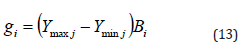
As in nature, the ith individual ( gi ) active range is determined by its own amplitude value ( Bi ). Equation 13 provides the active range computation.
v) Calculate Cartesian distance: To determine adjacent individuals in the sensing/active range, the distance between the ith individual and the remainder of the population must be computed. It is determined how far apart people i and h are using the Cartesian distance formula,
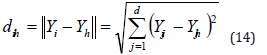
The electric fish algorithm uses equation 15 when at least one neighbor is present in the active sensing area; otherwise, when R = 0 , equation 16 is used
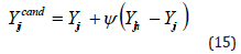
Where, h stands for a randomly selected individual from the ith individual’s neighbor set, that is, h∈R r, and ≤ ih dih gi .
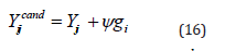
In equations 15 and 16,  stands for the potential position of the ith individual, and φ ∈[−1,1] is a random number chosen at random from a uniform distribution.
v. Renovating phase: In this electric fish algorithm, the electric fish generate weak electric signals for identifying objects and detecting the prey. It also helps them to navigate and communicate effectively with members of the same species in their often densely populated underwater habitats but the escaping capability from predators is not interpreted so it faced difficulties in handling large-scale optimization problems and slower convergence rates. To improve convergence rate and performance the jelly fish time control mechanism is merged with electric fish so it generates nematocysts to capture prey and defend themselves from potential threats. The combined equation’s mathematical formula is,
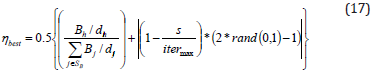
Where, h solutions of electric fish are determined from SB , s is the time index of jelly fish specified as the iteration number and itermax denotes the maximum iteration number.
Algorithm 1: Pseudo code for the proposed jelly electrophorus optimization
Result
A jelly electrophorus optimization method is suggested for the detection of breast cancer, and the model’s successes are evaluated in comparison to those methods to support their success.
Experimental setup
For conducting the breast cancer detection experiment, the Python programming language is employed, running on a Windows 10 operating system with access to 8GB of internal memory.
Dataset description
BreaKHis dataset (D1): This dataset has been curated to support breast cancer lesion research and analysis, utilizing histopathological images. At a microscopic level, these images depict breast tissue specimens treated with hematoxylin and eosin (H&E) stains. To aid in their classification, the dataset is segregated into two main groups: benign tumors, representing histologically benign lesions, and malignant cancers, representing histologically malignant lesions. A wide range of resolutions, spanning from low to high magnifications, is used to capture intricate details of the tissue structures. Each image is complemented by ground-truth annotations, precisely delineating regions of interest or specific cancerous areas. With a substantial volume of histopathological images, the dataset offers varying quantities of samples for each class, making it a valuable resource for breast cancer analysis and classification endeavors.
BreCaHAD dataset (D2)
The dataset known as BreCaHAD provides 162 breast cancer histopathology images, offering researchers an opportunity to enhance and evaluate their proposed methodologies. Within the dataset lies a wide array of malignant cases. The core objective centers around categorizing the histological structures found in these hematoxylin and eosin (H&E) stained images into six welldefined classes: mitosis, apoptosis, tumor nuclei, non-tumor nuclei, tubule, and non-tubule.
Evaluation metrics
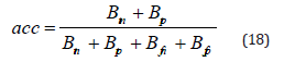
Accuracy: The accuracy serves as a measure of how often it correctly predicts both positive and negative cases. This metric is calculated as the percentage of cases accurately classified out of all occurrences in the dataset. A high accuracy indicates that the model successfully predicts both malignant and non-cancerous instances with precision.
Sensitivity: In the realm of medical diagnostics, sensitivity, also known as recall or the true positive rate, serves as a crucial metric in assessing a model’s ability to discern between positive instances, particularly those associated with malignancy. It is calculated as the ratio of true positives to the sum of true positives and false negatives. The model excels at accurately identifying cases of breast cancer when the dataset comprises such instances.
Specificity: The model’s specificity is contingent upon its capacity to discriminate proficiently between benign cases and all other negative instances. To calculate this metric, the ratio of true negatives to the sum of true negatives and false positives is employed. Due to its adeptness at accurately classifying nonmalignant cases, the model exhibits a high specificity value, effectively diminishing the likelihood of false positives.
Experimental results
The experimental results for detecting breast cancer using the JEO-3D deep CNN classifier are shown in Figure 4. The shown information includes the input image, datasets 1 and 2’s mean, median, standard deviation, and AlexNet, ResNet, and VGGNet.
Performance analysis
Evaluations of the proposed JEO-3D deep CNN model’s performance at various epochs, including those at 100, 200, 300, 400, and 500, demonstrate its usefulness. Utilizing TP, the performance is evaluated.
Performance analysis with TP for dataset 1: Figure 5 displays the performance analysis of the JEO-3D deep CNN model for dataset 1. At various epochs, the TP 90’s JEO-3D deep CNN accuracy is 94.53%, 94.93%, 95.33%, 95.73%, and 97.73%, respectively. Figure 5b shows the JEO-3D deep CNN sensitivity for the TP 90 at various epochs to be 85.59%, 94.70%, 95.27%, 95.85%, and 98.57%. Figure 5c shows that for the TP 90 at different epochs, the JEO-3D deep CNN specificity is 94.59%, 95.03%, 95.48%, 95.92%, and 98.13%, respectively.


Performance analysis with TP for dataset 2: Figure 6 displays the performance analysis of the JEO-3D deep CNN model for dataset 2. At various epochs, the TP 90’s JEO-3D deep CNN accuracy is 85.55%, 85.95%, 86.35%, 86.75%, and 88.75%, respectively. Figure 6b shows the JEO-3D deep CNN sensitivity for the TP 90 at various epochs to be 74.84%, 85.72%, 86.29%, 86.87%, and 90.32%. Figure 6c shows that for the TP 90 at different epochs, the JEO-3D deep CNN specificity is 85.61%, 86.05%, 86.50%, 86.94%, and 89.15%, respectively.
Comparative methods: K-Nearest Neighbor (KNN) Classifier (B1) [32], Support Vector Machine (SVM) Classifier (B2) [33], Decision Tree (DT) Classifier (B3) [34], Neural Network (B4) [35], bi-directional long short term memory (Bi-LSTM) (B5) [36], 3D Deep- CNN (B6) [37], 3D Deep- CNN With Jelly fish optimization (JFO) (B7) [38], 3D Deep- CNN With electric fish optimization (EFO) (B8) [39] is compared with JEO-3D deep CNN.
Comparative analysis with TP for dataset 1: In Figure 7, a comparative analysis of performance parameters for breast cancer detection in Dataset 1 is presented. When evaluating accuracy with a training rate of 90%, the suggested JEO-3D deep CNN exhibit an improvement rate of 0.43 compared to the 3D Deep-CNN with EFO Figure 7a. Moreover, the JEO-3D deep CNN demonstrate a higher increase rate of 0.60 in sensitivity when compared to the 3D Deep-CNN with EFO under the same training conditions of 90% (in Figure 7b. Likewise, when assessing specificity with a training rate of 90%, the suggested JEO-3D deep CNN showcase a notable increase rate of 0.47 over the 3D Deep- CNN with EFO Figure 7c.

Comparative analysis with TP for dataset 2: In Figure 8, performance metrics are utilized to juxtapose the results of breast cancer detection in Dataset 2. When evaluating accuracy with a training rate of 90%, the suggested JEO-3D deep CNN display a considerable improvement rate of 0.45 in comparison to the 3D Deep-CNN with EFO Figure 8a. Additionally, the suggested JEO-3D deep CNN exhibit a remarkable increase rate of 0.64 in sensitivity when compared to the 3D Deep-CNN with EFO under the same training conditions of 90% Figure 8b. Moreover, the proposed JEO-3D deep CNN demonstrate a comparable increase rate of 0.50 relative to the 3D Deep-CNN with EFO when assessing training specificity at 90% Figure 8c.
Comparative discussion
The existing methods are used to compare the results, and Table 1 shows the results. In this analysis, the assessment is conducted using 90% of the training data and 500 epochs for all approaches, ensuring optimal values for the comparison. The improvement measure unequivocally establishes the superiority of the proposed approach in accurately identifying breast cancer disease through histopathology images.

Conclusion
In this research jelly electrophorus optimization-based 3D density connected deep convolution neural networks (CNN) is developed for the identification of breast cancer using histopathology images. Pre-processing is done to enhance the qualities of the histopathological image after input is gathered. Then the feature extraction is performed through VGG-16, AlexNet, ResNet-101, statistical features. These features are concatenated using multiplied features patterns so it retains the unique characteristics of each feature, potentially leading to better model performance. Finally, these concatenated features are fed forwarded to 3D density connected 3D deep convolution neural networks (CNN) classifier it will automatically detect breast cancer effectively with the help of jelly electrophorus optimization. The classifier’s weights and bias are adjusted by the proposed jelly electrophorus optimization. When accuracy, sensitivity, and specificity of the results are examined, the proposed JEO-3D deep convolution neural networks (CNN) approach achieves values of 93.73%, 95.31%, and 94.14% for dataset 1 and 88.75%, 90.32%, and 89.15% for dataset 2, which is more effective. Pathologists can use the proposed breast cancer classification to deliver the appropriate care at an early stage and lower patient risk. For the real-time applications, the proposed method’s accuracy must be improved. Thus, a unique breast cancer classification system will be developed in the future to improve detection accuracy.
Ethics statements
The relevant informed consent was obtained from those subjects from open sources.
Credit author statement
Sagarkumar Patel conceived the presented idea and designed the analysis. Also, he carried out the experiment and wrote the manuscript with support from Rachna Patel. All authors discussed the results and contributed to the final manuscript. All authors read and approved the final manuscript.

Acknowledgment
I would like to express my very great appreciation to the coauthors of this manuscript for their valuable and constructive suggestions during the planning and development of this research work. This research did not receive any specific grant from funding agencies in the public, commercial, or not-for-profit sectors.
Declaration of interests
The authors declare that they have no known competing financial interests or personal relationships that could have appeared to influence the work reported in this paper.
References
- Reshm VK, Nancy Arya, Sayed Sayeed Ahmad, Ihab Wattar, Sreenivas Mekala, et al. (2022) Detection of breast cancer using histopathological image classification dataset with deep learning techniques. BioMed Research International 2022.
- Sharma, Shubham, Archit Aggarwal, Tanupriya Choudhury (2018) Breast cancer detection using machine learning algorithms. In 2018 International conference on computational techniques, electronics and mechanical systems (CTEMS) pp: 114-118.
- Chaurasia Vikas, Saurabh Pal (2017) A novel approach for breast cancer detection using data mining techniques. International journal of innovative research in computer and communication engineering 2(1).
- Tyson Rachel J, Christine C Park, J Robert Powell, J Herbert Patterson, Daniel Weiner, et al. (2020) Precision dosing priority criteria: drug, disease, and patient population variables. Frontiers in Pharmacology 11: 420.
- Gour Mahesh, Sweta Jain, T Sunil Kumar (2020) Residual learning-based CNN for breast cancer histopathological image classification. International Journal of Imaging Systems and Technology 30(3): 621-635.
- Charan, Saira, Muhammad Jaleed Khan, and Khurram Khurshid. Breast cancer detection in mammograms using convolutional neural network. international conference on computing, mathematics and engineering technologies (iCoMET) pp: 1-5.
- Bhardwaj, Arpit, Aruna Tiwari (2015) "Breast cancer diagnosis using genetically optimized neural network model. Expert Systems with Applications 42(10): 4611-4620.
- Gupta Varun, Megha Vasudev, Amit Doegar, Nitigya Sambyal (2021) Breast cancer detection from histopathology images using modified residual neural networks. Biocybernetics and Biomedical Engineering 41(4): 1272-1287.
- Bhise Sweta, Shrutika Gadekar, Aishwarya Singh Gaur, Simran Bepari, DSA Deepmala Kale (2021) Breast cancer detection using machine learning techniques. Int J Eng Res Technol 10(7): 2278-0181.
- Ragab, Dina A, Maha Sharkas, Omneya Attallah (2019) Breast cancer diagnosis using an efficient CAD system based on multiple classifiers. Diagnostics 9(4): 165.
- Maqsood, Sarmad, Robertas Damaševičius, Rytis Maskeliūnas (2022) TTCNN: A breast cancer detection and classification towards computer-aided diagnosis using digital mammography in early stages. Applied Sciences 12(7): 3273.
- Bourouis Sami, Shahab S Band, Amir Mosavi, Shweta Agrawal, Mounir Hamdi (2022) Meta-heuristic algorithm-tuned neural network for breast cancer diagnosis using ultrasound images. Frontiers in Oncology 12: 834028.
- Yan Rui, Fei Ren, Zihao Wang, Lihua Wang, Tong Zhang, et al. (2020) Breast cancer histopathological image classification using a hybrid deep neural network. Methods 173: 52-60.
- Memon, Muhammad Hammad, Jian Ping Li, Amin Ul Haq, Muhammad Hunain Memon, et al. (2019) Breast cancer detection in the IOT health environment using modified recursive feature selection. wireless communications and mobile computing 2019: 1-19.
- Chun Amy W, Stephen C Cosenza, David R Taft, Manoj Maniar (2009) Preclinical pharmacokinetics and in vitro activity of ON 01910. Na, a novel anti-cancer agent. Cancer chemotherapy and pharmacology 65: 177-186.
- Das Abhishek, Mihir Narayan Mohanty, Pradeep Kumar Mallick, Prayag Tiwari, Khan Muhammad, et al. (2021) Breast cancer detection using an ensemble deep learning method. Biomedical Signal Processing and Control 70: 103009.
- Zheng Jing, Denan Lin, Zhongjun Gao, Shuang Wang, Mingjie He, (2020) "Deep learning assisted efficient AdaBoost algorithm for breast cancer detection and early diagnosis." IEEE Access 8: 96946-96954.
- Khan Amir A, Jigar Patel, Sarasijhaa Desikan, Matthew Chrencik, Janice Martinez Delcid, et al. (2021) Asymptomatic carotid artery stenosis is associated with cerebral hypoperfusion. Journal of vascular surgery 73(5): 1611-1621.
- Boumaraf Said, Xiabi Liu, Zhongshu Zheng, Xiaohong Ma, Chokri Ferkous (2021) A new transfer learning-based approach to magnification dependent and independent classification of breast cancer in histopathological images. Biomedical Signal Processing and Control 63: 102192.
- Liu Qi, Chenan Zhang, Yue Huang, Ruihao Huang, Shiew Mei Huang, et al. (2023) Evaluating Pneumonitis Incidence in Patients with Non–small Cell Lung Cancer Treated with Immunotherapy and/or Chemotherapy Using Real-world and Clinical Trial Data. Cancer Research Communications 3(2): 258-266.
- Lilhore, Umesh Kumar, Sarita Simaiya, Himanshu Pandey, Vinay Gautam, "Breast cancer detection in the IoT cloud-based healthcare environment using fuzzy cluster segmentation and SVM classifier. In Ambient Communications and Computer Systems pp: 165-179.
- Hirra Irum, Mubashir Ahmad, Ayaz Hussain M, Usman Ashraf, Iftikhar Ahmed Saeed, et al. (2021) Breast cancer classification from histopathological images using patch-based deep learning modeling. IEEE Access 9: 24273-24287.
- Lu Si Yuan, Shui Hua Wang, Yu Dong Zhang (2022) SAFNet: A deep spatial attention network with classifier fusion for breast cancer detection. Computers in Biology and Medicine 148: 105812.
- Carvalho Edson D, O C Antonio Filho, Romuere RV Silva, Flavio HD Araujo, Joao OB Diniz, et al. (2020) Breast cancer diagnosis from histopathological images using textural features and CBIR. Artificial intelligence in medicine 105: 101845.
- Zebari, Dilovan Asaad, Dheyaa Ahmed Ibrahim, Diyar Qader Zeebaree, Mazin Abed Mohammed, et al. (2021) "Breast cancer detection using mammogram images with improved multi-fractal dimension approach and feature fusion. Applied Sciences 11(24): 12122.
- Viswanath V Harvin, Lorena Guachi Guachi, Saravana Prakash Thirumuruganandham (2019) "Breast cancer detection using image processing techniques and classification algorithms." EasyChair 2101 pp: 1-11.
- Sharma Shallu, Sumit Kumar (2022) The Xception model: A potential feature extractor in breast cancer histology images classification. ICT Express 8(1): 101-108.
- Afolayan, Jesutofunmi Onaope, Marion Olubunmi Adebiyi, Micheal Olaolu Arowolo, Chinmay Chakraborty, et al. (2022) Breast cancer detection using particle swarm optimization and decision tree machine learning technique. In Intelligent Healthcare pp: 61-83.
- Abbasniya Mohammad Reza, Sayed Ali Sheikholeslamzadeh, Hamid Nasiri, Samaneh Emami (2022) Classification of breast tumors based on histopathology images using deep features and ensemble of gradient boosting methods. Computers and Electrical Engineering 103: 108382.
- Ibrahim Rehab Ali, Laith Abualigah, Ahmed A Ewees, Mohammed AA AlQaness, Dalia Yousri, et al. (2021) An electric fish-based arithmetic optimization algorithm for feature selection. Entropy 23 9: 1189.
- Chou Jui Sheng, Dinh Nhat Truong (2020) Multiobjective optimization inspired by behavior of jellyfish for solving structural design problems. Chaos Solitons & Fractals 135: 109738.
- Assegie Tsehay Admassu (2021) An optimized K-Nearest Neighbor based breast cancer detection. Journal of Robotics and Control (JRC) 2(3): 115-118.
- Wang Haifeng, Bichen Zheng, Sang Won Yoon, Hoo Sang Ko (2018) A support vector machine-based ensemble algorithm for breast cancer diagnosis. European Journal of Operational Research 267(2): 687-699.
- Afolayan Jesutofunmi Onaope, Marion Olubunmi Adebiyi, Micheal Olaolu Arowolo, Chinmay Chakraborty, Ayodele Ariyo Adebiyi (2022) Breast cancer detection using particle swarm optimization and decision tree machine learning technique. In Intelligent Healthcare: Infrastructure, Algorithms and Management pp: 61-83.
- Alanazi Saad Awadh, MM Kamruzzaman, Nazirul Islam Sarker, Madallah Alruwaili, Yousef Alhwaiti, (2021) Boosting breast cancer detection using convolutional neural network. Journal of Healthcare Engineering.
- Li Li, Alimu Ayiguli, Qiyun Luan, Boyi Yang, Yilamujiang Subinuer, et al. (2022) Prediction and Diagnosis of respiratory disease by combining convolutional neural network and bi-directional long short-term memory methods. Frontiers in Public Health 10: 881234.
- Zhou Xiangrong, Takuya Kano, Hiromi Koyasu, Shuo Li, Xinxin Zhou, et al. (2017) Automated assessment of breast tissue density in non-contrast 3D CT images without image segmentation based on a deep CNN. In Medical Imaging 2017: Computer-Aided Diagnosis, 10134: 704-709.
- Martin Abadal, Miguel, Ana Ruiz-Frau, Hilmar Hinz, Yolanda Gonzalez Cid (2020) Jellytoring: real-time jellyfish monitoring based on deep learning object detection. Sensors 20(6): 1708.
- Yılmaz Selim, Sevil Sen (2020) Classification with the electric fish optimization algorithm. In 2020 28th Signal Processing and Communications Applications Conference (SIU) pp: 1-4.


