


Optimal Inventory Strategies for Pharmaceutical Products Incorporating Carbon Emissions
Priyan S*
Department of Mathematics, Mepco Schlenk Engineering College, India
Submission: April 25, 2019; Published: May 28, 2019
*Corresponding author: Priyan S, Department of Mathematics, Mepco Schlenk Engineering College, Virudhunagar 626005, Tamilnadu, India
How to cite this article: Priyan S. Optimal Inventory Strategies for Pharmaceutical Products Incorporating Carbon Emissions. Curr Trends Biomedical 003 Eng & Biosci. 2019; 19(2): 556008. DOI: 10.19080/CTBEB.2019.19.556008
Abstract
Heart failure (HF) is a major factor contributing to premature death in patients with established cardiovascular (CV) disease. Current cell therapies of HF based on at least two different approaches, in which stem cell transplantation and extracellular vesicles (EV) received from pre-treated cells, were used. Although in HF restoring cardiac function aimed improve survival is target of cell therapy, it is not yet yielded whether isolated EVs from circulating progenitor cells, induced pluripotent stem cells (iPSCs), human embryonic stem cells-derived CV progenitors (hESC-Pg) would be effective translators of reparative signals for cardiac repair. The short communication is depicted the role of different cell strategies in HF. It has emphasized lack of strong evidence of clinical advantages implanted EVs to human cells to iPSCs in HF requires comparison in large clinical trials.
Keywords: Heart failure; Cell therapies; Human stem cells; Human progenitors; Progenitor cell-derived extra vesicles
Abbreviations: HF: Heart Failure; CV: Cardiovascular; EV: Extracellular Vesicles; iPSCs: Induced Pluripotent Stem Cells; hESC-Pg: Human Embryonic Stem Cells- Progenitors; iPSCs: Induced Pluripotent Stem Cells
Introduction
A healthcare supply chain (HSC) consists of pharmaceutical wholesalers, pharmaceutical companies, hospitals, medical surgical distributors, etc. A stated one-third of hospital decision makers have belief their hospital supply chain is working at greatest point doing work well, but the other two thirds are discovering themselves one foot in fee-for-service and the other in value-based giving back of money. Many of these hospitals are not implementing the suitable supply chain management strategies. This is because most hospital administrators and pharmacy managers are doctors with expert knowledge in medicine and are not supply chain professionals. Unlike other industries, hospital administrators and pharmacy managers have to manage very complicated distribution networks and inventory management problems without proper guidance on efficient practices. Hence, given the high costs, constraints, and perishability of pharmaceuticals, more study is necessary to help health care managers in setting optimal HSC strategies. Recently few numbers of papers designed in the field of healthcare supply chain and inventory management (see [1-4]).
All steps from the supply of raw materials to the finished products can be covered in a supply chain connecting raw material suppliers, manufacturers, retailers, and the customer/hospital. Multi-echelon inventory management is the management of inventory and coordination of the distribution process at more than one level of a supply chain network. Kim [5] presented an explanation of an integrated supply chain management system developed to specifically address issues related to pharmaceuticals in the health care sector. Meijboom and Obel [6] addressed supply chain coordination for a pharmaceutical company with a multi-location and multi-stage operations structure. Amir et al. [7] developed a generalized network oligopoly model for HSC competition that takes into account product perishability, brand differentiation, and discard costs.
Lead time is an essential factor in any supply chain and inventory system. Liao & Shyu [8] devised a probabilistic inventory model in which lead time was considered as a decision variable. Several researchers extended this approach in integrated inventory models for lead time reduction (see [9-14]). Glock [13] studied alternative methods for controlling lead time and their impact on the safety stock and the expected total costs of a continuous review inventory control system. Moua et al. [14] introduced a more realistic lead time crashing cost in Glock [13]’s model. They proposed a modified integrated inventory model by adding the transportation time as a decision variable and assumed that there were two different safety stocks. They numerically showed that their modified model was more realistic than Glock [13] model.
Without considering carbon emissions in inventory management, the decision objective is usually set as the total cost minimization or the total profit maximization. However, taking emission reduction into account is likely to change the optimal solution and incurs additional cost. The health sector is a vital direct source of carbon emissions. It is also a highly heterogeneous segment that has seen both rapid increases and decreases in direct emissions from different sources over the last decade. A modification in inventory strategies is an effective way to decrease emissions so that carbon emission issues in inventory management have attracted attention in literature recently (see [15-19]).
This research explores the impact of both lead time and carbon emissions on the inventory decisions of a pharmaceutical company and hospital supply chain system. The paper assumes that the lead time for the first shipment consists of production time, setup and transportation time (nonproductive time), while the lead time for the rest of the shipments is only transportation time, and that lead time can be reduced by shortening nonproductive time and transportation time. The proposed study also adds the carbon emissions from transportation and storage into the account. The intention of our investigation is to obtain the optimal decisions (order quantity, production rate, nonproductive time, transportation time and total number of deliveries) to achieve hospital’s CSL while minimizing expected total cost, and to examine the effects of carbon emissions in the proposed healthcare system
Notations and Assumptions
To develop the proposed model, we adopt the following notations and assumptions which are similar to those used in Uthayakumar & Priyan [1].
Notations
I. For the Hospital D Expected demand rate in units per unit time σ The standard deviation of the demand in units per unit time A Ordering cost per order. h Holding cost per unit time Sp Procurement cost per unit Q Order quantity (finished products), a decision variable ω The expiration time (or shelf life), which is the length of time to the expiration date. θ(t) Deteriorating rate of finished products at time t, 0 ≤ θ(t) ≤ 1 L Length of lead time, a decision variable n The number of lots in which the product is delivered from the company to the hospital in one production cycle, a positive integer, a decision variable α Proportion of demands that are not met from stock so (1-α)is the service level X The lead time demand in units per unit time, a random variable II. For the pharmaceutical company P Production rate in units per unit time S Company’s setup cost per setup hp Holding cost per unit time.
Model Development
Hospital’s expected total cost
The hospital places an order after every Q units, therefore
for expected ordering cycle time of Q/D, the expected ordering
cost per unit time can be expressed by AD.
Q Similar to Glock [13],
we assume that the nonproductive time ts consists of m mutually
independent components tsr, i.e. The rth component
has a normal duration ur a minimum duration vr and a crashing
cost per unit time cr. For convenience, we rearrange cr such that
c1 ≤c2 ≤... ≤cm. Let ts
i represent the length of nonproductive time
with the components 1,2,...i crashed to their minimum duration,
then ts
i can be expressed as
The rth component
has a normal duration ur a minimum duration vr and a crashing
cost per unit time cr. For convenience, we rearrange cr such that
c1 ≤c2 ≤... ≤cm. Let ts
i represent the length of nonproductive time
with the components 1,2,...i crashed to their minimum duration,
then ts
i can be expressed as i=1,2,....m;and the lead time crashing cost per cycle is
  To gain the transportation time crashing cost C(tT) for the
shipments 1,2,3,....n, Similar to the assumptions made by Mou
[14], we assume that the lth component of the nonproductive time
ts is the setup time. Thus, the transportation time tT is composed
of m-1 mutually independent components, i.e.
To gain the transportation time crashing cost C(tT) for the
shipments 1,2,3,....n, Similar to the assumptions made by Mou
[14], we assume that the lth component of the nonproductive time
ts is the setup time. Thus, the transportation time tT is composed
of m-1 mutually independent components, i.e.
 We rearrange c1,c2,...,ci-1, cl+1,....cm in such
a way that 1 2 1 .
m c c c−′ ≤ ′ ≤≤ ′ Let tT
j be the length of the
transportation time with the components 1,2,3,...j crashed
to their minimum duration, then tT
j can be expressed as
We rearrange c1,c2,...,ci-1, cl+1,....cm in such
a way that 1 2 1 .
m c c c−′ ≤ ′ ≤≤ ′ Let tT
j be the length of the
transportation time with the components 1,2,3,...j crashed
to their minimum duration, then tT
j can be expressed as  1,2,3,..m-1. Hence, by
adopting the same technique used by Mou [14], the transportation
time crashing cost C(tT) for the shipments 2,3,...n
1,2,3,..m-1. Hence, by
adopting the same technique used by Mou [14], the transportation
time crashing cost C(tT) for the shipments 2,3,...n 
Thus the lead time crashing cost per unit time can be derived by ( ) ( 1) ( ) . s T D R t n R t nQ + − In addition, the reduction of lead time leads to a lower demand uncertainty, which may decrease the safety stock and the stock-out loss. Since , s T Q t t P + for the shipments 2,3,...n it might be beneficial to avoid holding additional safety stock by decreasing the reorder points. Consequently, Similar to Mou [14], we consider that there are two different safety stocks and reorder points for the first shipment and the shipments 2,3,...n. Then, the hospital’s expected holding cost per unit time isThus the lead time crashing cost per unit time can be derived by ( ) ( 1) ( ) . s T D R t n R t nQ + − In addition, the reduction of lead time leads to a lower demand uncertainty, which may decrease the safety stock and the stock-out loss. Since , s T Q t t P + for the shipments 2,3,...n it might be beneficial to avoid holding additional safety stock by decreasing the reorder points. Consequently, Similar to Mou [14], we consider that there are two different safety stocks and reorder points for the first shipment and the shipments 2,3,...n. Then, the hospital’s expected holding cost per unit time is

The hospital’s freshness index of a pharmaceutical product (perishable product) may be pretentious by time, temperature, dampness, refrigeration, etc. In practice, most pharmaceutical products have their own expiration dates. Feng et al. stated that health-conscious consumers prefer a perishable product with a longer remaining shelf life to a shorter one and they assumed that the customer’s freshness index is age-dependent. That is, itbegins with 1 at time 0, and then gradually degrades closer to 0 as the expiration date of the product approaches. Consequently, similar to Feng et al., we assume that the age-dependent freshness at time t is linearly decreasing from 1 at the beginning to 0 at the maximum lifetime m as follows:

Subsequently the expired finished products of the hospital for
the ordering cycle Q
D can be detected by 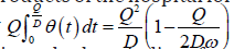 and disposed it with dispose cost Q2
ε since the hospital’s safety
stock inventories are sufficient to replace these expired finished
products. Then similar to the existing models, we consider the
reorder point
and disposed it with dispose cost Q2
ε since the hospital’s safety
stock inventories are sufficient to replace these expired finished
products. Then similar to the existing models, we consider the
reorder point  where kis the safety factor. Hence,
hospital’s expected total cost per unit time is composed of
ordering cost, holding cost, disposal cost and crashing cost, is
expressed by
where kis the safety factor. Hence,
hospital’s expected total cost per unit time is composed of
ordering cost, holding cost, disposal cost and crashing cost, is
expressed by

We assume in view of realistic healthcare system that the hospital has set a target service level in terms of the fill rate corresponding to the proportion of all product demands to be satisfied directly from available stock. Therefore, the Service Level Constraint (SLC) imposes a limit on the proportion of demands that are not met from stock. This can be mathematically expressed as

We consider the demand during lead time is normally
distributed with mean DL(P,Q) and DL(tT
), respectively, and standard deviation σ L( p,Q) and ( ), T σ L t
respectively, the safety stock is given by 1 . s s
S k t Q
P
= σ + The
expected shortage of the first batch shipment is given as 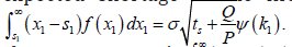 is the loss
function, which can be calculated as
is the loss
function, which can be calculated as  ϕ z dz ∞ = ∫ − where
ϕ (z) is the standard normal probability density function. Then,
the safety stock Ss can also be expressed as
ϕ z dz ∞ = ∫ − where
ϕ (z) is the standard normal probability density function. Then,
the safety stock Ss can also be expressed as 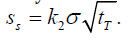 Now SLC can be written
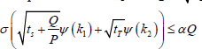
Pharmaceutical company’s expected total cost
Once the hospital orders a lot size of Q units, the company
produces the products in a lot size of nQ units with the setup cost
S in each production cycle of length nQ
D
with constant production
rate P units per unit time, and the hospital will receive the supply
in n lots each of size Q units. The first lot size of Q units is ready
for shipment after time
Q
P just after the start of the production.
During the production run time, nQ ,
P the company’s inventory is
building up at a constant rate, and simultaneously supplies a lot
of size Q units to the buyer on expected every Q
D units of time. Subsequently, during the non-production period the company
continues their shipments to the hospital on expected every Q
D
units of time (ordering cycle) until the inventory level falls to
zero. Based on the existing inventory models, the company’s
expected on hand finished products inventory is evaluated
as the difference of the company’s accumulated inventory
and the hospital’s accumulated inventory. Now, according to
Uthayakumar & Priyan [1], company’s accumulated inventory
is  and hospital’s accumulated inventory is
 units
units
Hence, based on Uthayakumar & Priyan [1], the
pharmaceutical company’s expected inventory is  Then,
the company’s expected holding cost per unit time
Then,
the company’s expected holding cost per unit time 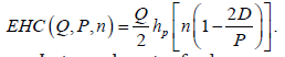
Let g0 denote fuel consumption of the unloaded (empty)
vehicle and g1 denote unit fuel consumption factor if the
supplier’s transportation vehicle is loaded with goods. This
research considers g0+g1Q captures amount of fuel consumption
for a one-way delivery from supplier to buyer. We assume that
backhaul is not used and return vehicles are empty, and that g0
is amount of the fuel consumption for the return trip. For one
inventory replenishment, the total amount of fuel consumption
2g0+g1Q. Hence, supplier’s average transportation cost per unit
of time is 
In this model, we measure the total amount of carbon emissions from transportation and storage. Thus, the associated amount of carbon emissions is designed by

In the above equation, Π1(Q,P,n) and Π2(Q,P,n) are the amounts of carbon emissions from transportation and storage, respectively. Then θ1 and θ2 are carbon emission factors for fuel and electricity. In Π2(Q,P,n), w0 and w1 are fixed and unit variable electricity consumption for storage. Accordingly, the company’s carbon emissions cost per unit time is derived by

Thus, the total cost function per unit time for the pharmaceutical company comprising of setup cost, holding cost, transportation cost and carbon emission cost, is expressed by

Then the joint expected total cost per unit time for the proposed pharmaceutical company and hospital integrated supply chain system is

Now our problem involves finding the optimal (Q,P,n,ts,tT) in a production cycle that minimize the joint expected total cost, JETC(Q,P,n,ts,tT) while satisfying SLC. That is, the primal problems of the proposed model is given as

Solution Procedure
The problems formulated in the previous section appear as constrained non-linear programming problems. To solve these problems, we temporarily ignore the SLC and relax the integer requirement on n, then we have to minimize joint expected total cost, JETC(Q,P,n,ts,tT)
Proposition 1: For fixed P,n,ts ϵ[ts i, ts i-1] and tT ϵ[ts i, ts i-1], JETC(Q,P,n,ts,tT) is convex in Q. Proof: Taking the first and second partial derivatives of JETC(Q,P,n,ts,tT) with respect to Q we have

Therefore, for fixed P,n,ts ϵ[ts i, ts i-1] and tT ϵ[ts j, ts j-1], is convex in Q. This completes the proof of Proposition 1. Result 1: For the given values of P,n,ts ϵ[ts i, ts i-1] and tT ϵ[ts j, ts j-1], by setting Eq. (2) equal to zero, we obtain the optimal Q and QH which minimize the JETC(Q,P,n,ts,tT):

Proposition 2: For fixed Q,n,ts ϵ[ts i, ts i-1] and tT ϵ[ts j, ts j-1], JETC(Q,P,n,ts,tT) is convex in P. Proof: Taking the first and second partial derivatives of JETC(Q,P,n,ts,tT) with respect to P, we have

Therefore, for fixed P,n,ts ϵ[ts i, ts i-1] and tT ϵ[ts j, ts j-1], JETC(Q,P,n,ts,tT) is convex in P. This completes the proof of Proposition 2. Result 1: For the given values of Q,n,ts ϵ[ts i, ts i-1] and ts ϵ[ts i, ts i- 1], by setting Eq. (4) equal to zero, we obtain the optimal P which minimize the JETC(Q,P,n,ts,tT): Proposition 3: For fixed Q,P, n JETC(Q,P,n,ts,tT) is concave in ts ϵ[ts i, ts i-1] and tT ϵ[ts j, ts j-1], i=1,2,...,m and j=1,2,....,m-1 Proof: Taking the second partial derivatives of JETC(Q,P,n,ts,tT) with respect to ts and tT respectively, we obtain the following Hessian matrix

It is clear that the Hessian matrix H is negative definite. Hence, JETC(Q,P,n,ts,tT) is a concave function with respect to ts and tT for fixed values of Q, P, n. This completes the proof of Proposition 3. Result 2: According to Proposition 3, for fixed Q,P,n,the minimum values of JETC(Q,P,n,ts,tT) and occur at the end points of the interval is ts ϵ[ts i, ts i-1]XtT ϵ[ts j, ts j-1] Proposition 4: For fixed Q,P,n,ts ϵ[ts i, ts i-1] and tT ϵ[ts j, ts j-1], JETC(Q,P,n,ts,tT) is convex in Proof: Taking the first and second partial derivatives of JETC(Q,P,n,ts,tT) with respect to we have

Therefore, for fixed Q and L ϵ[Li, Li-1], JETC(Q,n,L) is convex in n.This completes the proof of Proposition 4. Remark 1: The search for the optimal number of deliveries, is reduced to find a local minimum.
According to the Result 1, for fixed of P,n,ts ϵ[ts i, ts i-1] and tT ϵ[ts j, ts j-1], when the SLC is ignored, Eq. (3) gives optimal value of Q such that the joint expected total cost is minimum. Now, the SLC is taken into consideration and if for Q= QH then QH is the local minimum of JETC(Q,P,n,ts,tT) and SLC is inactive. Otherwise, optimal value of Q should be at least equal to ( ) ( ) ( ) SLC s 1 T 2 Q t Q k t k P σ α ψ ψ = + + which is greater than QH so that specified level of service can be achieved at minimum joint expected total cost and QSLC is the local minimum of JETC(Q,P,n,ts,tT). So, for fixed of P,n,ts ϵ[ts i, ts i- 1] and tT ϵ[ts j, ts j-1] the optimal Q is given by max{QH, QSLC}. Based on the convexity and concavity behavior of objective function with respect to the decision variables the following algorithm is designed to find the optimal values of the decision variables.
Algorithm
i. Step 1. Set n=1. ii. Step 2. For each ts i and ts j perform (2-1) to (2-5), i=0,1,...,m and j=0,1,...,m-1. • Step 2.1. Compute 1 2 ij P a a = and QH using Eq. (3). • Step 2.2. Compute p’ij and Q’H using Result 1 and Eq. (3) respectively. Repeat this step until convergence. Then set the optimal values po ij and Qo H • Step 2.3 Set Q=max{Qo H, QSLC}. If Qo H is maximum, then go to step 2.5, otherwise go to step 2.4. • Step 2.4. Compute po ij using QSLC then go to step 2.5. • Step 2.5. Compute the corresponding JETC(Qij,Pij,n,ts,tT) by putting Q= Qo H and p= po ij in Eq. (1). iii. Step 3. Let JETC(Q*,P*,n,ts*,tT*)=min(i=0,1,...,m-1), (j=0,1,...,m-1) JETC(Qij,Pij,n,ts,tT). Then the optimal solution for fixed values of n is (Q*,P*,n,ts*,tT*). iv. Step 4: Set n= n+1 v. Step 5: Repeat Steps 3 and 3 to get MJETC(Q*,P*,n,ts*,tT*). vi. Step 6: If JETC(Q*,P*,n,ts*,tT*) ≤ JETC(Q*,P*,n-1,ts*,tT*) then go to Step 4, otherwise go to Step 7 vii. Step 7: Set (Q*,P*,n,ts*,tT*)=(Q*,P*,n-1,ts*,tT*). Then (Q*,P*,n,ts*,tT*) is optimal solution to achieve target CSL which minimize joint expected total cost.
Conclusion
In this paper, we designed a new algorithm to achieve the target customer service level while minimizing system cost of the proposed healthcare supply chain system. We provided an optimal inventory policy through mathematical model to modify the operators in order to reduce carbon emissions. This research explores the impact of both lead time and carbon emissions on the inventory decisions of a pharmaceutical company and hospital supply chain system.
References
- Uthayakumar R, Priyan S (2013) Pharmaceutical supply chain and inventory management strategies: optimization for a pharmaceutical company and a hospital. Operations Research for Health Care 2(3): 52-64.
- Priyan S, Uthayakumar R (2014) Optimal inventory management strategies for pharmaceutical company and hospital supply chain in a fuzzy-stochastic environment. Operations Research for Health Care 3(4): 177-190.
- Susarla N, Karimi IA (2018) Integrated production planning and inventory management in a multinational pharmaceutical supply chain. Computer Aided Chemical Engineering 41: 551-567.
- Savadkoohi E, Mousazadeh M, Ali Torabi S (2018) A possibilistic location-inventory model for multi-period perishable pharmaceutical supply chain network design. Chemical Engineering Research and Design 138: 490-505.
- Kim D (2005) An integrated supply chain management system: a case study in healthcare sector. In: Lecture Notes on Computational Science 3590: 218-227.
- Bert Meijbooma, Børge Obel (2007) Tactical coordination in a multi-location and multi-stage operations structure: a model and a pharmaceutical company case. Omega 35(3): 258-273.
- Amir H Masoumi, Min Yu, Anna Nagurney (2012) A supply chain generalized network oligopoly model for pharmaceuticals under brand differentiation and perishability. Transportation Research E 48(4): 762-780.
- Liao CJ, Shyu CH (1991) An analytical determination of lead time with normal demand. International Journal of Operations Production Management 11: 72-78.
- Pan JCH, Yang JS (2002) A study of an integrated inventory with controllable lead time. International Journal of Production Research 40: 1263-1273.
- Liang Yuh Ouyang, Kun Shan Wu, Chia Huei Ho (2004) Integrated vendor buyer cooperative models with stochastic demand in controllable lead time. International Journal of Production Economics 92(3): 255-266.
- Mohammad A Hoque, Suresh K Goyal (2006) A heuristic procedure for an integrated inventory system under controllable lead-time with equal or unequal sized batch shipments between a vendor and a buyer. International Journal of Production Economics 102(2): 217-225.
- Hoque MA (2007) An alternative model for integrated vendor buyer inventory under controllable lead time and its heuristic solution. International Journal of Systems Science 38: 501-509.
- Glock CH (2012) Lead time reduction strategies in a single-vendor–single-buyer integrated inventory model with lot size-dependent lead times and stochastic demand. Int J Production Economics 136: 37-44.
- Moua Q, Cheng Y, Liao H (2017) A note on lead time reduction strategies in a single-vendor-single-buyer integrated inventory model with lot size-dependent lead times and stochastic demand. International Journal of Production Economics 193: 827-831.
- Jaber MY, Glock CH, El Saadany AMA (2013) Supply chain coordination with emissions reduction incentives. International Journal of Production Research 51: 6982.
- Hammami R, Nouira I, Frein Y (2015) Carbon emissions in a multi-echelon production-inventory model with lead time constraints. International Journal of Production Economics 164: 292-307.
- Jauhari WA, Pamuji AS, Rosyidi CN (2014) Cooperative inventory model for vendor-buyer system with unequal sized shipment, defective items and carbon emission cost. International Journal of Logistics Systems and Management 19: 163-186.
- Sunil Tiwari, Yosef Daryanto, Hui Ming Wee (2018) Sustainable inventory management with deteriorating and imperfect quality items considering carbon emission. Journal of Cleaner Production 192: 281-292.
- Qingguo Bai, Yeming Gong, Mingzhou Jin, Xianhao Xu (2019) Effects of carbon emission reduction on supply chain coordination with vendor-managed deteriorating product inventory. International Journal of Production Economics 208: 83-99.


