Abstract

This study develops a five-stage true stress–strain model for ASTM A992 and CSA G40.21 350W structural steels to address the limitations of conventional engineering stress–strain relationships in large- deformation analysis. Standard uniaxial tensile tests were conducted to establish baseline mechanical properties, and the model was formulated using a power law to describe the strain-hardening phase and a weighted combination of the power law and linear hardening to capture the post-ultimate strength response. Calibration was performed by aligning analytical and numerical predictions with the experimental tensile data, and validation was achieved through simulations of perforated tension coupons, which showed strong agreement between predicted and experimental load–deformation behavior. The results demonstrate that the proposed model can capture the complete stress–strain response from elastic deformation through strain hardening, post-ultimate behavior, and fracture, providing improved material characterization for these steel grades and offering potential for extension to other steels, particularly where accurate modeling of necking and fracture is required.

Keywords:Material Models for Steel; True stress- strain relations; Power-law Hardening; Large Deformation; FE Analysis

Introduction

The accurate characterization of material behavior under different loading conditions forms the foundation of reliable structural design and advanced numerical analysis. In both mechanical engineering and materials science, one of the most important representations of this behavior is the true stress-strain curve, which provides a detailed description of how materials deform and harden beyond the elastic limit [1,2]. Unlike the conventional engineering stress-strain curve, which is expressed in terms of the original cross- sectional area and gauge length of a tensile specimen, the true stress-strain curve reflects the instantaneous values of stress and strain during deformation [3]. This distinction becomes critical once a material yields and enters the plastic range, where its performance governs the structural capacity, ductility, and eventual failure. For ductile materials such as structural steel, the true stress-strain relationship is indispensable in understanding and predicting plastic deformation, strain hardening, and ultimate failure, all of which are vital to designing safe and efficient structures [4-6].

The engineering stress–strain curve is sufficient for basic characterization in the elastic range and early plastic deformation, but its utility diminishes as the material approaches and surpasses the ultimate tensile strength (UTS). The reason lies in the assumptions underlying engineering definitions: stresses are calculated using the original cross-sectional area, and strains are measured with respect to the initial gauge length. Once necking initiates, these assumptions no longer hold. At the onset of necking, a localized instability develops in which the specimen’s cross-sectional area decreases more rapidly at the necked region than elsewhere. This results in a non-uniform stress and strain distribution, accompanied by triaxial stress states that are not captured by engineering definitions [7,8]. Consequently, the engineering curve inaccurately portrays the true mechanical response in the post-UTS region, where accurate data is most crucial for failure and fracture prediction [9].

The significance of this issue is well recognized. While the conversion of engineering stress and strain to true stress and strain is straightforward during the uniform deformation stage, the same cannot be said once necking occurs. After UTS, determining the true stress-strain curve becomes a complex task, requiring techniques that can capture localized strain fields and account for non-uniform stress distributions. Conventional methods, such as using extensometers and load frames, are incapable of providing reliable data beyond the necking point. To overcome this limitation, researchers have relied on advanced experimental approaches, including digital image correlation (DIC), highresolution strain mapping, and inverse analysis methods based on finite element modeling [10-12]. While effective, these approaches demand sophisticated equipment, specialized expertise, and significant resources, which limit their accessibility for routine engineering practice. As a result, a persistent gap exists between the theoretical need for complete true stress–strain curves and the practical difficulty of obtaining them.

This gap carries important implications for finite element analysis (FEA), which is widely used in structural and mechanical design to simulate material behavior under complex loading conditions. Reliable simulations require material models that accurately capture the entire stress–strain history, particularly the post-necking behavior that dictates failure modes and energy absorption capacity. Without robust post- necking data, FEA models risk underestimating or overestimating structural performance, leading to unsafe designs or overly conservative assumptions [13,14]. For critical infrastructure and advanced applications, such inaccuracies can have severe consequences. Therefore, developing a methodology that provides engineers with a practical and reliable way to obtain the full true stress– strain curve is both scientifically necessary and professionally valuable.

To address this challenge, the present study proposes a simple and cost-effective methodology for deriving the complete true stress–strain curve of structural steel from data that can be obtained in a conventional tensile test. The approach begins with the reliable pre-necking data obtained from direct conversion of engineering to true stress–strain values. To extend this curve beyond the UTS, the methodology incorporates two critical data points that are readily measurable: the stress and strain at themaximum load and the values at fracture. These points, when combined with computational tools, provide the framework for estimating the post-necking behavior. The study explores and evaluates several post-necking strain hardening models, including linear extrapolation, power-law formulations, and a weighted average approach. Each model is constrained by fundamental mechanical principles, particularly the Considère criterion, which governs the onset of necking, ensuring that the extrapolated curves remain physically consistent with material behavior [15,16].

Among the models investigated, the weighted average method emerges as a particularly effective approach for bridging the gap between measured data and theoretical expectations. By blending multiple strain- hardening representations and calibrating them against the fracture data, this model provides a robust and realistic description of the material’s deformation up to failure. Importantly, the methodology does not rely on specialized instrumentation or advanced testing, making it accessible to engineers and researchers with limited resources. This simplicity does not come at the expense of accuracy, validation against experimental data demonstrates that the proposed method captures the essential features of post-necking behavior with consistency and reliability [17].

The contributions of this study are therefore twofold. First, it introduces a methodology that makes the complete true stress– strain curve attainable through standard tensile testing procedures combined with modest computational analysis. Second, it provides engineers with a practical tool for enhancing the fidelity of numerical simulations, particularly finite element models of structural steel components subjected to large deformations and extreme loads. By closing the gap between experimental limitations and simulation requirements, the proposed approach enables more accurate predictions of structural performance, energy absorption, and failure mechanisms.

In summary, the accurate determination of the true stress– strain relationship is central to advancing both materials science and structural engineering practice. The challenges associated with post-necking characterization have historically limited the accessibility of complete curves, particularly in routine engineering applications. This study addresses the problem by proposing and validating a practical, low- cost methodology that leverages conventional tensile data, critical fracture parameters, and carefully chosen strain-hardening models. The results not only demonstrate the feasibility of this approach but also highlight its significance in enhancing the reliability of numerical simulations. Ultimately, this research offers a bridge between experimental simplicity and computational sophistication, contributing to safer, more efficient, and more predictive engineering design.

Research Significance

This research investigates the mechanical behavior of solid and perforated steel tension members, focusing on how flange holes, bolted connections, and metal-forming processes affect their performance. The study introduces a versatile framework whose principles can be applied not just to steel, but to a wide range of metals. This versatility is crucial for advancing both structural engineering and materials science, as it enables the development of innovative and resilient designs that can withstand diverse loading and environmental conditions. By providing a precise model for metal behavior under tension, this research allows engineers to design structures with superior reliability and longevity. The study’s findings are poised to set new standards in modern construction and manufacturing, making a significant contribution to the evolution of material science and engineering practices. The insights gained from this work can influence the design and application of materials across various industries.

Test Program

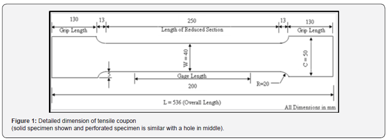
The test program aimed to establish the mechanical properties of ASTM A992 and CSA G40.21 50W/350 W steel grades [6] by conducting tensile tests on standard coupons extracted from the rolled beams of these materials. Tensile coupons were fabricated according to the dimensions and guidelines specified in ASTM A370-17 [5]. Figure 1 illustrates the detailed dimensions and characteristics of standard tensile coupons. The design includes a cross-sectional reduction strategically implemented to localize failure through necking, followed by fracture within the reduced section.

To ensure precise strain measurement, two MTS-type extensometers were attached to the reduced section. The first extensometer with a gauge length of 200 mm was used to capture the overall strain across the coupon. A second extensometer, with a shorter gauge length of 50 mm, was used to assess the mechanical properties within the elastic range. The minimal weight of the extensometers relative to the specimens ensured that any out-ofplane deformation under direct tension loading was negligible, allowing accurate and reliable data collection.

Test Matrix

The test matrix consisted of sixteen flange coupons and 12 web coupons. For each steel grade (A992 and 350 W), three identical solid coupons were selected from both the flanges and web sections to determine their mechanical properties. The remaining ten flange coupons and six web coupons were perforated with holes of varying diameters at their centers to investigate the effect of these perforations on the tensile behavior. The holes were strategically placed in the highly stressed central region of the coupons to maximize their impact on tensile performance. These holes were created using a slow cold-drilling process to minimize any material alterations around the holes. It is important to note that the effect of the hole- making process on fracture behavior is beyond the scope of this study. For flange coupons, hole diameters were chosen to achieve net area-to-gross area (A_n/A_g) ratios ranging from 0.9 to 0.5 in increments of 0.1. The hole diameters of the web coupons were selected to achieve the A_n/A_g ratios of 0.9, 0.7, and 0.5.

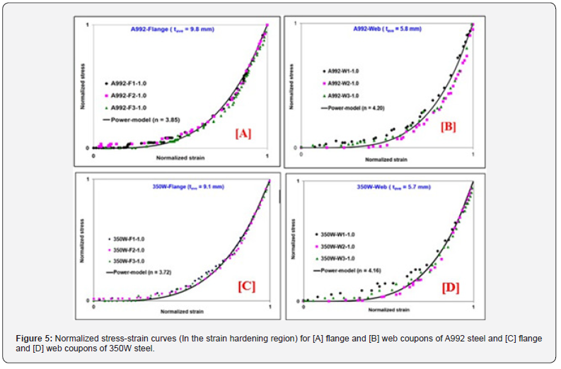
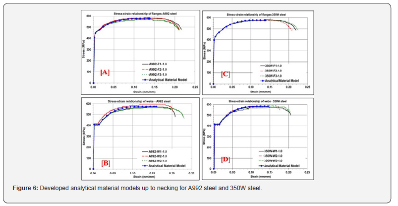
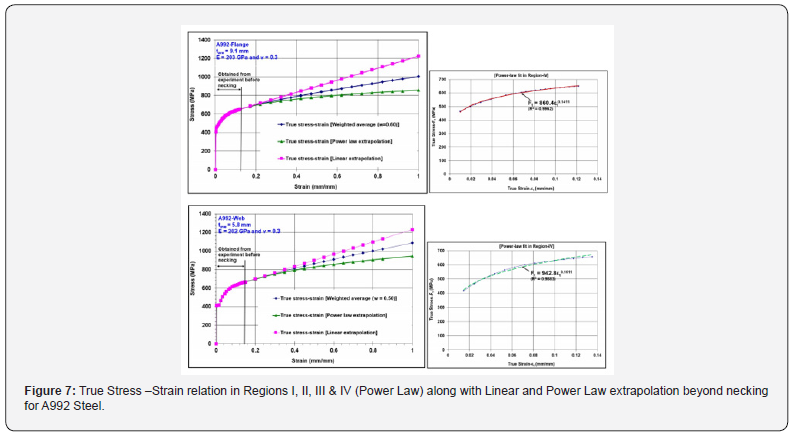
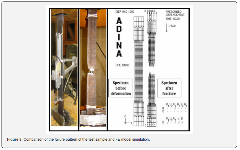
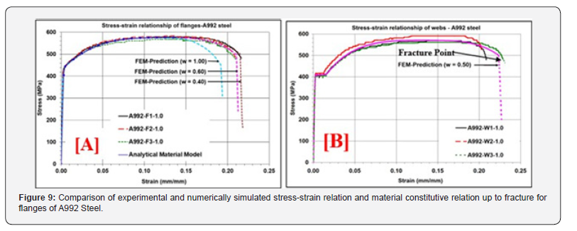
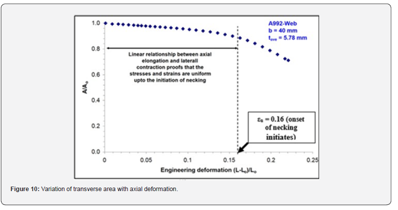
Figure 2 illustrates some of the test coupons and the corresponding failure modes observed in both solid and perforated samples. To ensure accuracy, the width and thickness of the coupons were measured multiple times within the reduced cross-section. These measurements were used to calculate the initial cross-sectional area of each specimen precisely. The next section outlines the detailed methodology for conducting the tensile tests.

Test Procedure

All tension tests were conducted using a Tinius Olsen machine with an axial load capacity of 600 kN, operated using controlled mechanical (screw) power. The machine was calibrated prior to the initiation of tensile tests. The following steps outline the procedure in detail:
i. Alignment and Grip: The gripping or holding device of the testing machine to transmit the load from the heads of the machine to the specimen under test was initially positioned vertically and precisely centered with respect to the grips located on the loading platforms of the machine. This was performed to ensure a secure hold and eliminate any bending or twisting with the vertical axis of the specimen at the beginning and during the test.
ii. Extensometer Setup: Two extensometers were employed in this procedure: one with a gauge length of 200 mm and the other with a gauge length of 50 mm. An extensometer with a gauge length of 200 mm played a pivotal role in determining the overall stress-strain relationship between engineering stress and engineering strain. At the same time, a 50 mm gauge length extensometer was used to determine the parameters in the elastic range, including the elastic modulus (E), proportional limit (Fpl), and strain corresponding to the proportional limit (ɛ_pl).

iii. Loading Sequence: The testing speed was carefully calibrated according to ASTM A370 guidelines [5] to ensure accurate results. In the elastic range, up to the yield point, a loading rate of 0.008 mm/s was employed to prevent premature plastic deformation, which was significantly lower than the ASTM recommended maximum of 1/16 inch/min (~0.026 mm/s). Once the yield point was surpassed, and throughout the strainhardening phase up to the ultimate load, the rate was increased to 0.042 mm/s, which was still well below ASTM’s upper limit of 1/2 inch/min (~0.212 mm/s). Beyond the ultimate load, the initial loading rate of 0.008 mm/s was reinstated during the postultimate phase to fracture, effectively minimizing the strain rate effects during necking and fracture and ensuring the integrity of the test results [18]. Previous studies have clearly shown that higher strain rates result in lower fracture strains [19-21].

This comprehensive testing protocol was executed to make sure to acquire a detailed understanding of the behavior of the material throughout its various phases, from elastic deformation to ultimate failure. The collection of extensive data under a controlled load rate ensured that sufficient data were collected to establish reliable test results, which will eventually be used for numerical simulations and finite-element- based predictions on a larger scale.

(R_p = 1.0 for drilled hole and U = 1.0, as no shear lag)

Test Results – Solid Coupons

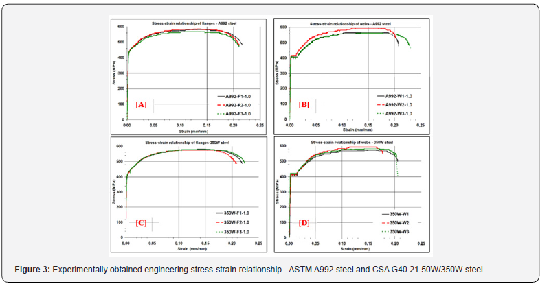
Figure 3 illustrates the engineering stress versus strain relationships obtained based on the solid tensile coupons from the flanges and webs of the W310x39 beam section made of ASTM A992 steel grade and CSA G40.21 50W/350 W steel grade.
• A992 Steel: Table 1 summarizes the mechanical properties of the tensile coupons from the flanges and webs of the A992 steel. The average yield strength (F_y) and ultimate strength (F_u) of the A992 flange were 445 and 577 MPa, respectively, with a yield-to-ultimate strength ratio (F_y/F_u) of 0.77. The strains at the ultimate strength (ε_u) and fracture (ε_f) were 13.8% and 20.8%, respectively. For the A992 web, Fy and F_u were 409 and 573 MPa, respectively, with an F_y/F_u ratio of 0.71. The average Young’s modulus (E) is 203 MPa for the flange and 202 MPa for the web.
• 350W Steel: The mechanical properties of tensile coupons from 350 W steel are also shown in Table 1. The average F_y and F_u values of the flange were 428 and 578 MPa, respectively, with an F_y/F_u ratio of 0.74. The ε_u and ε_f values are 13.8% and 22.0%, respectively. For the 350 W web, F_y and Fu were 416 and 582 MPa, respectively, with an F_y/F_u ratio of 0.71. The average Young’s modulus (E) is 213 MPa for the flange and 201 MPa for the web.

These results provide critical insights into the mechanical properties of the A992 steel section for both flange and web coupons. Data on yield and ultimate strength, as well as strain at failure, are fundamental for understanding the behavior of the material and for further analysis and design considerations in engineering applications.

Test Results - Perforated Coupons

The presence of holes in the middle of the tension members resulted in notably distinct behaviors compared to their solid counterparts with uniform cross sections. This divergence in behavior was clearly observed in the overall stress-strain relationships that were established experimentally. Tension members with perforations exhibit a non-uniform stress distribution, which may be attributed to stress concentration effects in the vicinity of the hole region. This phenomenon indicates that the presence of perforations in a tension member, in the form of those used for connection via bolts, led to early yielding around these holes. This early yielding caused the loaddeflection relationships to exhibit an early non- linear behavior.
• A comparison of gross section yielding and net section fracture criteria: The behavior of perforated tension members is highly dependent on the size of the hole(s) relative to the gross cross-section of the member. For example, the member may reach a gross section yield load (A_gF_y) if the holes are small with respect to the gross cross section, the member may reach a gross section yield load (A_gF_y). However, as the size of the holes increases, the member tends to fail because of net section fracture before reaching the capacity for gross section yielding (A_gF_y).
• Yield ratio (Y) to define the failure modes: It has been long proved that when A_nF_u>A_gF_y or A_n>YA_g, gross section yielding occurs prior to the net area fracture as the dominant failure mode, where Y is defined as the yield-to-ultimate strength ratio (F_y/F_u). Therefore, it can be concluded that, for members with identical geometries and perforations, the yield-to-ultimate strength ratio (Y) is the dominant factor in determining the anticipated failure mode.

The experimental results showed that the behavior of the tension members was significantly different for members with different [A_n /A_g] ratios. Factors such as the size of perforations, yield ratio (Y), and gross- to-net areas determine the failure mode prior to the others in terms of gross section yielding and/ or net section fracture. This is a fundamental understanding of the structural behavior of tension members with perforations to ensure that the structural components behave as expected under various loading conditions.

Results Summary

Table 2 presents important data related to the tensile tests, including the yield load (P_y = A_gF_y), ultimate load (P_u), P_u/P_y ratio, maximum average stress across the net section (Fun = P_u/A_n), and strength ratios based on perforated versus solid samples (F_un/F_u) of the same steel grade.

The summary results indicate that tension members or coupons with an A_nF_u/A_gF_y ratio greater than 1.0 achieved an ultimate load (P_u) exceeding the yield load Py (=A_gF_y). Conversely, coupons with an A_nF_u/A_gF_y ratio of less than 1.0 fractured before reaching Py. The ultimate strengths of the perforated samples (F_un) were observed to be 2-8% higher than those of the solid samples (Fu). This finding aligns with Fisher et al.’s study [22,38], which suggested that the presence of holes in axial tension members may limit free lateral contraction, potentially leading to slightly higher strengths in perforated samples than in solid ones. However, no consistent pattern emerged in the strength ratios (A_nF_u/A_gF_y) in this study, likely because of factors such as variations in material properties, geometric imperfections, and differences in holemaking practices [21-25].

Development of Analytical Material Model

The mechanical characteristics of steel elements can be established using a standard tensile test procedure. These test results are mostly informative within the small elastic-plastic deformation range. However, this method has limitations and provides little information when the material undergoes significant deformation, particularly beyond the post ultimate range. Within post ultimate range, the material often exhibits strain softening owing to the necking phenomenon, followed by fracture failure in ductile materials such as steel. Necking refers to a localized reduction in the cross-sectional area as the material is stretched. The use of the original cross-sectional area in stress calculations is problematic under these conditions [21,26].

As necking progresses, the stress-strain distribution becomes non-uniform and complex. Determining the magnitude of these quantities in the necked region has become increasingly difficult [21, 27-28]. Recognizing the significant changes in the geometric configuration of a specimen during high levels of axial deformation, it is essential to account for these changes to accurately describe the response of steel materials throughout the deformation process up to fracture [27]. To achieve a comprehensive understanding, a constitutive model is required, which requires a true stress-strain curve for the material. The relationship between the true stress and strain can be derived directly from the initial engineering stress-strain relationship [21,38].

This relationship is described by equations F_t = F_e (1 + ε_e) and ε_t = ln(1 + ε_e), where F_t represents the true stress, ε_t is the true strain, F_e is the engineering stress, and ε_e is the engineering strain. These relationships between the true and engineering quantities are based on two fundamental assumptions: 1) stresses were uniformly distributed across the specimen, and 2.) material flows with negligible volume change. However, it is important to note that, as necking occurs and non-uniform stressstrain distributions manifest beyond the onset of necking, these equations are no longer applicable in the post-ultimate range. In these later stages, the material behavior becomes more complex and challenging to describe using simple engineering stress-strain relationships. More advanced models and analysis techniques are required to capture the full range of behaviors.

Development of Regions for A992 and 350W Steels

In the analysis of the material’s stress-strain behavior, Figure 4 illustrates the stress-strain relationship in terms of engineering measurements, which is used as the mechanical property of many steels used in structural applications. Additionally, the dashed line represents the true stress-strain relationship. This analysis divides the overall stress-strain behavior into five distinct regions, each with its specific characteristics, as described below:
• Region-I: This is an elastic region, and the relationship between engineering stress and strain is linear and follows Hooke’s law. Stress is directly proportional to the strain, and the material returns to its original shape when the load is removed (up to a proportional limit). The 0.01% strain offset method is a common technique for determining stress at the proportional limit. The stress (F_e) at the proportional limit can be expressed as F_e=E_εe when F_e< F_pl, where E is the initial elastic modulus of a material. The relationship between the true stress and true strain from the engineering stress and engineering strain can also be converted into F_t=F_e (1+ ε_e) and ε_t =ln(1+ ε_e).
• Region-II: In the region between the proportional limit (F_pl) and yield limit (F_y), the relationship between the stress and strain can be characterized by the tangent modulus (E_t). This relationship can be related to F_e = E_t ε e as long as F_pl < F_e < F_y. E_t represents the tangent modulus, which can be calculated as E_t = [(F_y − F_pl)]/[(ε_y-ε_pl)]. Furthermore, it is important to note that, as mentioned earlier, the relationships F_t = F_e(1+ε_e) and ε_t=ln(1 + ε_e) remained valid throughout the deformation process.
• Region-III: In the stress-strain behavior of materials, particularly metals, after yielding begins, there may be a yield plateau during which the stress remains relatively constant at the yield stress, F_y. This yield plateau was observed in the region ε_y < ε_e < ε_sh. The stress in this region is considered constant and equal to the yield stress F_y. The material exhibited plastic deformation without a significant increase in the stress. The ratio of εsh to ε_y, denoted as “m,” characterizes the relationship between the strain at the onset of hardening and the strain at the yield point. This equation is defined as m=εsh/εy. When m=1, there was no distinct or sharp yield plateau observed. In this case, the behavior of the material transitions directly from the elastic region to hardening without a significant plateau. It is important to note that the relationships F_t= F_e(1 + ε_e) and ε_t=ln(1 + ε_e) remained valid even in this region.
• Region-IV: Following the yield plateau, ductile materials, such as steel, enter the strain-hardening phase, enabling materials to gain higher strength. Region IV encompasses the strainhardening range, extending to the ultimate strength, where the test specimen might begin to show necking. Although this region involves a non-linear stress-strain relation, the noted relationship still holds: F_t=F_e (1+ ε_e) and ε_t =ln(1+ ε_e). Note that in the strainhardening region (Region-IV), materials often show a power-law relationship that describes the engineering stress-strain behavior [29-30]. This relationship is widely used in materials science to capture the non-linear analytical behavior of materials during strain hardening. Thus, the power-law equation can be expressed as F_e = k(ε_e)ⁿ. The constants, k and n are material-specific and describe the response of the material during strain hardening. The value of n, known as the strain- hardening exponent, quantifies the rate at which the material hardens. A higher n shows a more rapid increase in strength during strain hardening. To determine the values of these constants, the stress-strain data obtained from the experimental test results were transformed and normalized. The process of transforming and normalizing the data allows for the estimation of k and n, yielding a mathematical description of the behavior of the material in Region-IV.

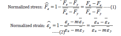
where 𝐹̅_𝑢 and 𝐹̅_𝑦 are the average ultimate and yield strengths, respectively, and ε̄_𝑢 and ε̄_𝑦 are the average strains corresponding to the ultimate yield strengths. Upon transforming the stressstrain data into a normalized form, the coefficient k becomes unity, leaving only one unknown n to be found. Hence, the power model used to describe Region IV can be expressed as:

In Figure 5, the stress-strain relationship for the flange and web coupons of the A992 and 350 W steel grades within the strain-hardening region (Region-IV) is illustrated. The data were obtained experimentally from a few coupons. The purpose of this exercise was to compile the stress-strain data, which will serve as the basis for developing a suitable analytical model for subsequent finite element (FE) studies as part of the research program. To determine the value of a least-square fit was performed. This involves adjusting the value of n in the equation to best match the normalized stress-strain test data corresponding to Region- IV. The least-squares fit is a mathematical optimization technique used to find the best-fitting curve for the experimental data by minimizing the sum of the squares of the differences between the model’s predictions and the actual data. Overall, Figure 5 and the process of determining n contributed to the development of a more precise and reliable analytical model for the subsequent FE model.

Simplifying Equation 3 yields the analytically derived engineering stress - engineering strain relationship in the strainhardening region, as follows:

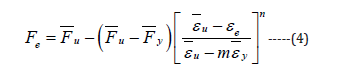
Figure 6 illustrates the analytical material models developed for the flanges and web coupons of the A992 steel sections. The models were constructed to reflect the behavior of the steel specimens based on the experimental data. This means that they are grounded in the actual mechanical response of the material, as observed in tests up to the ultimate strength, prior to the initiation of necking.

• Region-V represents the post-ultimate strength behavior of a material, which can be challenging to characterize owing to the complexity of the material behavior in this phase, particularly during necking and just before fracture. An experimental-numerical iterative approach was employed in this study to address these challenges. Moreover, this procedure was utilized to establish a suitable constitutive relation beyond post ultimate range until the fracture of the A992 and 350 W steel grades in this investigation.

Development of Numerical Model Using FE Simulation in Region-V

The method adopted in this study involved iteratively simulating tensile test results obtained from solid samples using Finite Element Method (FEM)-based analyses. The purpose of this exercise was to establish the parameters that can be used to develop a true stress-strain relationship. The reason for this approach being iterative is that the entire stress-strain relationship during necking is not known, which necessitates a trial-and-error procedure at various strain intervals until a good correlation with the experimental results has been achieved. This trial-and-error approach makes the method computationally intensive and timeconsuming. Therefore, the true stress-true strain relationships during necking were numerically established based on both a lower and upper bound for the true stress-strain function in this region. These two bounds were used as a weighted average to establish a true stress- true strain relationship that represents the load-extension curve obtained experimentally [20]. The powerlaw fit is the lower bound that characterizes the strain-hardening region of the flow curve, and the upper bound represented by a linear hardening model was employed in this study.

Figure 7 shows the upper and lower bound models, along with the weighted model, to represent the true stress-true strain relationship in Region V, the post-ultimate strength region. A breakdown of the contents is presented in Figure 7.
• Linear Hardening Model: In context of Figure 7, the linear hardening model is expressed as F_t = a₀ + a1ε_t, where a₀ = F_ut (1 − ε_ut) and a₁ = F_ut. The terms Fut and εut represent the true strength and true strain, respectively, corresponding to the ultimate engineering strength. Hence, F_t=F_ut (1+ ε_t - ε _ut). This model is suitable for linearly extrapolating the true stress-strain curve beyond the necking point.
• Power Law Hardening Model: As described under Region-IV, a power-law hardening model can be expressed in the form of F_t = F_ut (ε_t /n)n, where ‘n’ can be obtained by doing a linear regression analysis of true stress-true strain curve of strain hardening portion established through the analytical approach as described in Region-IV.
• Weighted Average Method: The weighted average method can be used to establish the true stress- true strain relationship in Region-V and can be expressed in the form of

• Weighting Constant (w): The weighted average model incorporates a weighting constant, denoted as ‘w.’ This constant is unknown and is required to be determined through an iterative process. The range of ‘w’ is between 0 and 1 (0 < w < 1.0). The weighted model combines an upper bound (for constant or linear strain-hardening extrapolation, obtained when w=1) and a lower bound (for power-law strain-hardening extrapolation, derived when w=0). These bounds provide the boundaries for the true stress-true strain relationship within Region-V.
• Iterative Numerical Approach: To establish a suitable value for the weighting constant ‘w,’ an iterative numerical approach, based on Finite Element (FE) modeling and analysis, of solid tensile tests was implemented to achieve a good correlation between test and predicted curves.

Numerical simulation of tensile test results - FE analysis

Many real-world scenarios involve complex loading conditions, and accurate stress-strain modeling is necessary to simulate the behavior of a material under these conditions. This characterization is typically based on uniaxial tensile tests, which provide fundamental data for understanding the response of a material to loading. However, in ductile materials, the occurrence of necking can lead to the loss of a homogeneous material response because the subsequent nonuniform deformation complicates the behavior of the material. This, in turn, makes the prediction of local characterization difficult, particularly for applications such as metal forming, analysis of bolted connections in a steel structure, analysis of corroded steel pipes, and bulk forming operations such as drawing, extrusion, and rolling.

Note that the data collected from a standard tensile test would provide only sufficient information pertaining to the material behavior up to the initiation of necking. Beyond necking, the data collected from such tests may only provide an average stress-strain relationship. These average data might not accurately capture the complex behavior of the material in large-strain applications. The limited data available beyond necking can seriously constrain the use of FE in applications involving significant deformation. This limitation, as noted by Ling in 1996 [20], highlights the need for more advanced methods to accurately characterize the material behavior in the post-necking region.

This study investigated and developed a material model that closely represents ASTM A992 and CSA G40.21 50W/350 W steels. The most important aspect of this study is how the approach described herein can be extended to any steel grade or ductile material. Thus, the determination of the weight constant w involves an iterative process. The iterative process aimed to adjust the weight constant w within the FE model to achieve the best possible agreement between the calculated load-extension curve (F*(e, w)) and the experimental load-extension curve (F(e)). This iterative approach fine-tunes ‘w’ to minimize errors and improve the accuracy of the FE model.

Finite Element Modeling Procedure

The numerical simulation of the tensile test coupon involved the use of 4-node shell elements, each equipped with six degrees of freedom per node, capable of accommodating finite strains and suitable for both thick- and thin-shell structures [31]. These elements were integrated with 2 × 2 points in the mid- surface (in the r-s plane) and three Gauss numerical integration points through the thickness (in the t- direction) to ensure accurate modeling. In addition, this shell element can be efficiently used with plastic multilinear material models for large-displacement/ large-strain analyses [27]. A geometric imperfection, represented by a half-sine wave with a maximum amplitude of 0.1% of the width (40 mm), was introduced along the gauge length to mimic the diffuse necking. The analysis considered both geometric and material nonlinearities, utilizing the von Mises yield criterion and the isotropic hardening rule for plasticity. The boundary conditions included a full restraint on one end and uniform displacement at the other end, emulating the tensile test conditions. Note that a true stress-strain relationship was derived analytically from engineering stress-strain curves (in Regions I, II, III, and IV) based on standard tensile tests, ensuring an accurate representation of material behavior in various deformation stages.

A fine mesh was employed to accurately capture the highly localized necking phenomenon and strain gradients in the central region of the sample. Within this central region, square elements measuring 2 × 2 mm were used. This mesh size was previously proven to be effective in dealing with large displacement and strain problems when using the 4-node shell element, as proven in a previous study by Khoo in 2000 [32]. In areas away from the necking region, a coarser mesh was sufficient given that the strain demands in these locations were significantly smaller than those in the central region, where necking initiation and fracture occurred.

The loading type employed in the analysis involves applying a uniform displacement in small increments. Initially, a prescribed increment of 0.15 mm was introduced using ADINA [33]. However, beyond the ultimate load, the ADINA finite element program autonomously adjusted the increment size to ensure continued loading until the model fractured. This adaptive approach was necessary because the stress and strain fields became more complex after initiation of the necking phenomenon. The automatic time-step increment facility available in ADINA was used to control the displacement increments.

In Region V, the material model required an additional data point (E1) to accurately represent the true stress-strain relationship, as shown in Figure 4. As discussed, a weighted average method was used to establish the true stress-true strain relation for Region V. Earlier studies have also revealed that the localized fracture strains for structural steel under uniaxial tensile loads can vary between 80% and 120% [32]. The estimated fracture strain (ε_ft) associated with the experimental results, as shown in Figure 2, was in the range of 65-75%. In this study, for consistency and comparison, the true strain at point E₁ was set to ε_ft = 100% [21]. Figure 8 provides a visual comparison, highlighting a photograph of a test specimen after failure along with the corresponding finite element models. This additional data point helps ensure an accurate representation of the material behavior in Region V, especially during the post-ultimate strength phase.

To illustrate the impact of the selection of w on the simulation outcomes, three different values were considered in the finite element simulation: w = 1.00, 0.60, and 0.40. Figure 9 displays the resulting finite element model (FEM)-predicted responses compared with the experimental responses for the A992-flange samples. When w was set to 1.00, representing extrapolation based purely on a power-law hardening rule, the FEM response appeared to fall below the experimental curve beyond the onset of necking, with a lower strain at fracture. Conversely, for w set at 0.40, the overall trend of the numerical curve was slightly above that of the experimental curve beyond the onset of necking, with a slightly larger strain at fracture. After a careful review of these scenarios, the value of w was determined to be 0.60, as it resulted in the FEM response showing good agreement with the averaged test results. Although finding the right value for w to reproduce an experimental stress-strain curve typically involves a trial-anderror approach, in this study, a suitable value was determined after a few trials.

FE results summary for simulation of solid coupon test

The model parameters were derived from the experimental results and included three identical flange coupons and three identical web coupons. In this study, FE simulations of tensile tests were conducted, and weighing constants of w=0.6 and w=0.5, closely replicated the stress-strain curve obtained from the flanges and webs of ASTM A992 steel grade. The numerical fracture stresses showed a maximum deviation of 3%, whereas the fracture strain differed by a maximum of 5% when compared to the corresponding experimental values. A similar procedure was adopted to determine the weighting constants for the 350 W steel grade. Table 3 summarizes the weighting constants and material models established for the flanges and webs of ASTM A992 and 350 W steel grades.

Table 4 compares the stresses and strains at fracture of the standard coupons simulated using the FE model with the mean experimental values of the three solid samples. The numerical stresses and strains at fracture exhibited a maximum deviation of 2% when compared to the experimental values for ASTM A992 steel, whereas the deviation was as high as 5% for CSA G40.21 350 W steel. In general, the numerically simulated mean stress-strain curves demonstrated strong agreement with their experimental counterparts.

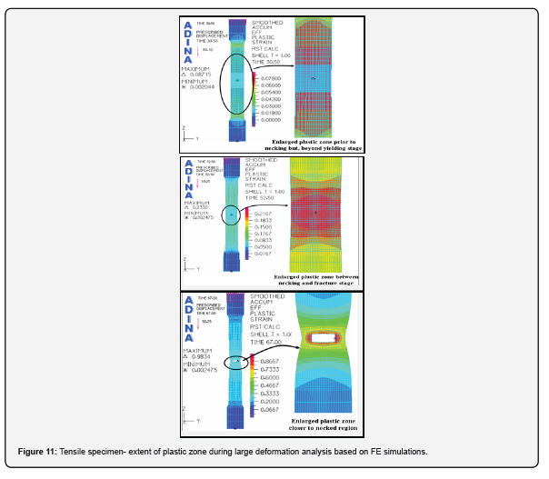
Figure 10 illustrates the evolution of stresses and strains in a tensile specimen, capturing the transition from uniform to nonuniform deformation following the onset of necking. During the initial stages of loading, up to the point of necking initiation, the inward transverse displacement increases uniformly along the specimen’s length. Beyond this stage, however, the displacement localizes exclusively within the necked cross-section, clearly reflecting the concentration of deformation in this region. This behavior highlights the highly localized nature of stresses and strains once necking begins, indicating that the specimen can no longer be considered to deform uniformly. A more detailed progression of strain in a specimen with a reduced section is presented in Figure 11, spanning the elastic and plastic stages of deformation. While the central reduced region undergoes plastic deformation, the wider ends of the specimen remain within the elastic range throughout the loading process. Notably, at a final strain of approximately 98%, only the necked region continues to deform plastically, whereas all other regions unload elastically. This finding is consistent with the simulations performed in this study, where a 100% strain at the ultimate fracture stage was assumed to replicate the experimental coupon response.

FE Analysis and Verification of Perforated Samples

The material constitutive relations, calibrated through experimental testing and validated by numerical analyses of standard coupon specimens, were subsequently employed to simulate the load–deformation behavior of perforated samples. These perforated specimens, extracted from both the flange and web regions of the A992 structural steel section, provided a representative evaluation of the material response in conditions closer to actual structural details. Figure 12 presents a direct comparison between the finite element (FE) predictions and the corresponding experimental results for these perforated samples. As shown, the FE-derived mean stress-strain curves closely follow the experimentally measured responses over the full deformation history, including the elastic, yielding, and strain- hardening phases. The agreement is particularly notable in the post-yield region, where accurate representation of strainhardening behavior is critical for capturing the true deformation capacity of structural elements. Minor deviations observed at higher strain levels can be attributed to localized effects around the perforations, such as stress concentration and constraintinduced triaxiality, which are inherently more challenging to capture with continuum FE models. Nevertheless, the overall consistency between the numerical and experimental responses underscores the robustness of the adopted constitutive relations and their suitability for modeling perforated sections.

Table 5 summarizes the experimental and FEM-predicted ultimate stress values for the perforated coupons fabricated from ASTM A992 and CSA G40.21 350W steels. The results demonstrate that the proposed material model achieves a close correlation with the experimental data, with the ratio F_{u^Exp/Fu^FEM generally falling within a ±3% deviation. For the A992 specimens, the FEM predictions slightly underestimated the ultimate strength in the F- series specimens (ratios ranging from 1.00 to 1.03), while the W-series specimens showed similarly close agreement, with ratios between 0.99 and 1.01. These results indicate that the model is capable of accurately capturing both the uniform section response and the localized effects introduced by perforations. A992 steel grade.}

The performance for the 350W specimens was even more consistent. The F-series specimens exhibited a nearly perfect correlation, with F_{u^Exp/Fu^FEM values equal to 1.00 across all perforation sizes, demonstrating that the model can replicate the load-carrying capacity of this steel grade with high fidelity. The W-series specimens also showed strong agreement, although a slightly larger deviation was observed for the largest perforation size (350W-W-0.5), where the FEM underpredicted the ultimate strength by approximately 4% (Fu^Exp/Fu^FEM=0.96). Nevertheless, this deviation remains within acceptable engineering limits. This level of agreement provides confidence in the predictive capability of the FE models for assessing the structural performance of steel members with geometric discontinuities, such as web openings or service holes, under realistic loading conditions.}

Table 6 presents a comparison between the test results and calculated values based on the CAN/CSA S16-24 code [35] for the perforated samples. As expected, the test results consistently surpassed the code- predicted ultimate load by an average of 40%. This discrepancy can be attributed to the code’s inherently conservative approach, which permits only 75% of the ultimate tensile strength to be considered for a safe design. This conservatism accounts for various uncertain factors such as holemaking practices, shear lag effects, and residual stresses. Similarly, Table 7 compares the test results with the current AASHTOLRFD 2020 code provisions for direct-tension members [34]. As anticipated, the test results exceeded the code-predicted values by 32% on average. This variance is again due to the conservative design philosophy of the code, which considers only 80% of the ultimate tensile strength to ensure safety.

Conclusion

The contributions of this study are threefold. First, it demonstrates that advanced FE modeling techniques, when paired with calibrated constitutive relations, can reliably capture the entire load-elongation behavior of ductile steels, including fracture. Second, it validates the predictive capability of the proposed material model, showing that parameters derived from solid coupon tests can effectively replicate the performance of perforated specimens with deviations typically within 3%. Third, it establishes a generalizable framework that can be extended to other steel grades and potentially to other ductile metallic materials. By bridging experimental testing, analytical modeling, and numerical simulation, this research provides both practical tools for structural engineers and theoretical insights into the mechanics of ductile fracture. The key findings and conclusions drawn from this study are as follows:

i. Advanced FE Modeling: Systematic finite element (FE) modeling techniques have been shown to accurately replicate the load-elongation behavior of ductile materials under direct tension, extending reliably to the point of fracture.
ii. Predictive Material Models: Material models derived from numerical simulations of standard tensile coupons effectively predict the load-deformation behavior of perforated coupons, with minor deviations primarily occurring at the final elongation, thereby demonstrating their practical applicability.
iii. This study introduces an innovative five-stage approach for developing a material constitutive relation for ductile steel materials subjected to axial tension. The stages are as follows.

• Region I: Linear Elastic Range In initial phase, the material behaves elastically, meaning that the deformation is fully recoverable upon unloading. The strain (ɛ_e) remained below the proportional strain threshold (ɛ_pl). The force (F_e) is directly proportional to the strain, defined by Hooke’s Law as F_e = E_ɛe, where E is the Young’s modulus. The true stress (F_t) was then calculated as F_t = F_e(1 + ɛ_e), and the true strain (ɛ_t) was derived using the relationship ɛ_t = ln(1 + ɛ_e).

• Region II: Nonlinear Elastic Range As material approaches yielding, its behavior becomes nonlinear. This occurs when the strain exceeds the proportional strain threshold (ɛ_pl) but is still less than the yield strain (ɛ_y). The force in this range is a combination of the elastic and plastic responses, represented as F_e = (E - E_t)ɛ_pl + E_tɛ_e, where E_t is the tangent modulus. The true stress and strain were similarly adjusted as F_t = F_e(1 + ɛ_{e) and ɛt = ln(1 + ɛe).}

• Region III: Yield Plateau Range Once the material yields, it enters a plateau where the stress remains constant despite the increasing strain. This range extends from the yield strain (ɛ_y) to strain-hardening threshold (ɛ_sh). During this phase, the true stress remains at the yield stress (F_y) and is expressed as F_t = Fy(1 + ɛ_e), with the true strain continuing to be ɛ_t = ln(1 + ɛ_e).

• Region IV: Strain Hardening Range Beyond the yield plateau; the material begins to strain hardening, meaning that it strengthens as it deforms. This phase occurs between the strain-hardening threshold (ɛ_sh) and the ultimate strain (ɛ_u). The stress increases according to a power-law model: F_t = F_ut(ɛ_t/ɛ_ut)ⁿ, where F_ut is the ultimate tensile strength, ɛ_ut is the ultimate true strain, and n is the strain-hardening exponent.

• Region V: Post-Ultimate Strength Range After material reaches its ultimate tensile strength, it begins to soften until fracture occurs. This final stage, extending from the ultimate strain (ɛ_u) to the fracture strain (ɛ_f), was modeled using a weighted average method that combined experimental and finite element (FE) simulation data.

The true stress was calculated as F_t = F_ut[w(ɛ_t/ɛ_ut)ⁿ + (1-w) (1 + ɛ_t − ɛ_ut)], where w is a weighting factor determined through calibration.

In summary, the study advances the state of knowledge on the tensile behavior of perforated steel members by introducing a calibrated five-stage constitutive model that captures the complete stress–strain response up to fracture. The proposed approach is particularly relevant for structural applications where perforations and localized stress states govern performance, and where conventional models fail to offer sufficient accuracy. Beyond its immediate application to A992 and 350W steels, the framework has broader implications for enhancing structural reliability assessments, informing design codes, and supporting advanced simulation-based evaluations of steel structures under extreme loading conditions.

References

1. Faridmehr R, Osman SA, Shah A, Azlan SA (2014) Correlation between Engineering Stress-Strain and True Stress-Strain Curve. American Journal of Civil Engineering and Architecture 2(1): 1-7.
2. Dieter GE (1986) Mechanical Metallurgy (3^rd) McGraw-Hill.
3. ANSYS Innovation Space (2020) Engineering Strain and True Strain. ANSYS Education.
4. Callister WD, Rethwisch DG (2021) Materials Science and Engineering: An Introduction (11^th). Wiley.
5. ASTM (A370-22) Standard Test Methods and Definitions for Mechanical Testing of Steel Products. ASTM International.
6. CSA (2021) General Requirements for Rolled or Welded Structural Quality Steel. Canadian Standards Association.
7. Bridgman PW (1952) Studies in Large Plastic Flow and Fracture. McGraw-Hill.
8. Tvergaard V, Needleman A (1984) Analysis of the cup-cone fracture in a round tensile bar. Acta Metallurgica 32(1): 157-169.
9. ASTM (E646-16) Standard Test Method for Tensile Strain-Hardening Exponents (n-Values) of Metallic Sheet Materials. ASTM International.
10. Sutton MA, Orteu JJ, Schreier H (2009) Image Correlation for Shape, Motion and Deformation Measurements: Basic Concepts, Theory and Applications.
11. Coppieters S, Cooreman S (2011) Identification of post-necking hardening behavior using digital image correlation. International Journal of Solids and Structures 48(9): 1244-1253.
12. Hora P, Tong L, Berisha B (2013) Inverse methods for the identification of post-necking material behavior. International Journal of Material Forming 6(1): 93-105.
13. Seif M, McGinnis MJ, Mirmiran A (2016) Finite element modeling of structural steel components under large deformations. Structures 5: 95-106.
14. Besson J (2010) Continuum models of ductile fracture: A review. International Journal of Damage Mechanics 19(1): 3-52.
15. Yasnikov IS, Vinogradov A, Estrin Y (2014) Revisiting the Consider criterion from the viewpoint of dislocation theory fundamentals. Scripta Materialia 76: 37-40.
16. Stoughton TB, Zhu X (2004) Review of theoretical models of the strain-based forming limit curve for sheet metals. Journal of Engineering Materials and Technology 126(4): 413-420.
17. Zhao L, Kuwabara T, Peng X (2023) A simple procedure for the post-necking stress-strain curves of anisotropic sheet metal. International Journal of Mechanical Sciences 248: 108191.
18. Jaquess KT, Frank K (1999) Characterization of the Material Properties of Rolled Sections.
19. Liu A (2005) Mechanics and Mechanisms of Fracture: An Introduction. ASM International.
20. Ling Y (1996) Uniaxial True Stress-Strain after Necking. AMP Journal of Technology 5: 37-48.
21. Arasaratnam P (2008) The Effects of Flange Holes on Flexural Behavior of Steel Beams, a Doctoral dissertation, McMaster University, ON, Canada.
22. Fisher JW, Struik JHA (1974) Guide to Design Criteria for Bolted and Riveted Joints, John Wiley and Sons, New York, USA.
23. Aldo M, Pietro F, Filippo B, Raffaele L (2024) Post-necking and damage modelling of steel structural components: A Comprehensive Sate of the Art. Journal of Structural Engineering 321: 118931.
24. Iman Faridmehr, Mohd Hanim Osman, Azlan Adnan, Ali Farokhi Nejad (2014) Correlation between Engineering Stress-Strain and True Stress-Strain Curve. American Journal of Civil Engineering and Architecture.
25. Yazhi Zhua , Amit Kanvindeb, Zuanfeng Pan (2019) Analysis of post-necking behavior in structural steels using a one dimensional nonlocal model. Journal of Engineering Structures 180: 321-331.
26. Zhou T, Roy SS, Wang J, Nie X, Chen H (2020) Parametric Study on the Structural Behavior and Failure Mechanism of Skewed Inverted-T Bent Caps. Journal of Bridge Engineering.
27. Mackenzie AC, Hancock JW, Brown DK (1977) On the Influence of State of Stress on Ductile Failure Initiation in High Strength Steels. Engineering Fracture Mechanics 9: 167- 188.
28. Cabezas EE, Celentano DJ (2004) Experimental and numerical analysis of the tensile test using sheet specimens. Finite Element in Analysis and Design 40: 555-575.
29. Arasaratnam P, Satya SR, Jiaji W (2025) A state-of-the-art review of current code provisions for girders with flange holes. Structures 71: 108155.
30. Bjorhovde R, Engstrom FM, Griffis GL, Kloiber AL, Malley OJ (2001) Structural Steel Selection Consideration: A Guide for Students, Educators, Designers, and Builders. ASCE, Virginia, USA.
31. Qin X, Roy SS, Xiong H, Mo YL, Kong Q (2022) Multidirectional crack monitoring of concrete structures using 3D piezoceramic sensing array. Structural Control and Health Monitoring 10: e3041.
32. Hollomon JH (1945) Tensile Deformation. Transactions of the American Institute of Mechanical Engineering 162: 268-277.
33. Bathe KJ (1996) Finite Element Procedures, Prentice Hall, Englewood Cliffs, NJ, USA.
34. Khoo AH (2000) Ductile Fracture of Steel Uniaxial True Stress-Strain after Necking. AMP Journal of Technology 5: 37-48.
35. Adina RD (2007) Adina 8.4 Version User Manual. Watertown, USA.
36. Aashto (2020) LRFD Bridge Design Specifications, Ninth Edition (2020) American Association of State Highway and Transportation Officials, Washington, DC, USA.
37. CSA (2024) Limit States Design of Steel Structures, CAN/CSA-S16-24, Canadian Standard Association, ON, Canada.
38. Oz Y, Wang J, Roy SS, Zhang S, Joshi B, et al. (2022) Finite-Element Simulation and Cost-Benefit Analysis of Full-Scale Skewed Inverted-T Bridge Caps with Traditional and Skew Reinforcements. Journal of Bridge Engineering 27(7).