Submission: February 19, 2024; Published: February 27, 2024

*Corresponding Author: Sai Nethra Betgeri, Department of Computer Science, University of Louisville, 2301 S 3rd St, Louisville, KY United States

How to cite this article: Sai Nethra Betgeri*, Shashank Reddy Vadyala and John C Matthews. Probability and Consequence of Failure for Risk-Based Asset Management of Wastewater Pipes for Decision Making. Civil Eng Res J. 2024; 14(4): : 555892. DOI 10.19080/CERJ.2024.14.555892

Abstract

Within wastewater systems, it is imperative to determine the probability of failure (POF) and consequence of failure (COF) for pipes as integral components of a risk-based decision framework. Identifying the POF and COF enables decision-makers to make more informed choices regarding the planning of current and future rehabilitation and replacement projects. This study introduces a novel risk assessment model employing Continuous-Time Markov Chain (CTMC) for calculating the probability of failure and utilizing the weighted average, coupled with the weighted rating method, to assess the consequences of failure. Subsequently, the model was applied to a wastewater network in northeastern Louisiana as a case study. The findings illustrated the POF of pipes for the next 200 years, with Corrosion, Soil Type, and Waste Type identified as the primary factors contributing to increased costs of failure. Approximately 40% of pipes necessitate moderate to high costs, and 7% of pipes require high costs. Unfortunately, validation of the developed model was hindered by insufficient data.

Keywords: Continuous-Time Markov Chain; Weighted Average; Probability of Failure (POF); Consequence of Failure (COF)

Introduction

Aging wastewater infrastructure is a growing source of concern for utilities all over the country. The US water sector earned a worrying C- Report [1] but got an upgrade from the previous D score [2], US wastewater sector earned a worrying D+ ASCE [3] in the most recent Infrastructure Report Card. Over the next 25 years, $271 billion will be needed to run and manage these networks at the required level of operation. In addition, it is expected that demand for wastewater collection and treatment will increase by 23% by the end of 2032 [3]. Risk-based asset management entails recognizing the most critical properties to pursue the most effective action in rehabilitating and replacing these structures. Potential wastewater pipe failures that could cause significant economic, social, and environmental costs are prevented by prioritizing replacing assets with the highest failure risk. Additionally, the most important pipes, which will be in worst, will be repaired or replaced first before any severe failure occurs [4-7]. Determining the chance or probability of failure (POF) and the consequence of failure (COF) are two steps involving pipe risk failure.

The likelihood that the pipe will fail is necessary for a full decision framework (POF). To effectively evaluate the risk of failure for a POF at any given moment, having pertinent information is essential. With this knowledge, decision-makers can better strategize and allocate funds for ongoing and future rehabilitation and replacement projects. Up until now, POF models have been employed to calculate pipe probabilities after one year using DTMC. However, there is a need to extend this approach to calculate probabilities for larger diameters using CTMC and to determine probabilities based on pipe age, also utilizing CTMC.

The initial element within the modeling framework for risk analysis, namely the probability of pipe failure, can be derived from historical data obtained through pipe inspections. Various methodologies, including statistical models Chughtai and Zayed [8], Markov chain models [9-11], and artificial neural networks Najafi and Kulandaivel [12] are employed to assess the likelihood of failure in water and wastewater pipes. Furthermore, predictive variables such as pipe material, age, length, depth, diameter, and past incidents of failure contribute to the determination of pipe failure probabilities.

The second component of the risk analysis modeling framework is determining wastewater pipes’ consequences. Unfortunately, many works cannot be found on estimating the consequence of failure because it involves both direct and indirect costs. Water Research Foundation report on the COF stressed the importance of assessing the indirect cost of COF along with the direct cost of COF. The report stressed the importance of assessing the COF using a triple bottom line (TBL). A TBL assesses the impact using economic, social, and environmental costs. The utilities bear economic costs, the customers indirectly bear social costs because of traffic delays or rerouting or service outages, and environmental impacts are contamination of soil and water. However, assessing wastewater pipe COF using the TBL approach is a rather challenging task due to the multiple and complex aspects related to determining economic, social, and environmental consequences. The difficulty lies in quantifying these consequences due to the different measurement scales of these impacts. Previously the other Consequence of failure (COF) model is COF model developed using AHP has factors related to pipe characteristics, external characteristics, and hydraulic characteristics under social, economic, and environmental impact but it has limitations because of the subject matter expert. Whenever subject matter expert opinion is varying the COF model consequence is getting changed and whenever factors are added or removed entire AHP process must be redone.

Objective

The main goal of this study is to introduce a decisionmaking framework based on risk assessment for planning the rehabilitation and replacement of wastewater pipes in the context of pipe renewal. The Probability of Failure (POF) and Consequence of Failure (COF) model encompasses a total of 12 factors. The POF model is constructed using Continuous Time Markov Chain (CTMC), while the COF model is established based on a weighted average approach. Notably, this research stands out due to its inclusive rating system, which incorporates the widely accepted PACP methodology in the industry. The outline of the framework is presented in Figure 1.

Materials and Methods

Probability of Failure:

In the first step, the factors under the criteria in Comprehensive rating K-NN Betgeri et al. [13], as shown in Figure 2, and the final comprehensive ratings calculated using K-NN are used for the CTMC model.

CTMC Model:

A CTMC is a stochastic model that describes a system with a countable state space that enters state i at time s and stays there for a random amount of time. In this study, the stochastic process {X(t), t ≥ 0} is a CTMC that describes the uncertain condition of a wastewater segment over time. This is called the sojourn time, and it is exponentially distributed, with parameter qi (qi ≥ 0) as shown in Eq. 1 [14]:

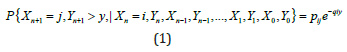
where

• Yn=Sn-Sn-1 (n ≥ 1) is the nth sojourn time

• Sn is the time of the nth (n ≥ 1) transition

A CTMC, {X(t), t ≥ 0}, has an embedded DTMC, {Xn, n ≥ 0}, for which transition probabilities, given the sojourn times, can be expressed as shown in Eq.1 [14].

After spending exponentially distributed time in state i, the system jumps to state j with probability pij at a time t. According to Kulkarni [14], the sojourn time and the new state depend only on the current state, state i, and not on any past states before time t. Thus, history impacts the future outcome through the current and present state of the system.

To find and solve the transition probability matrix at time t, P(t), of such a process, the differential equation shown in Eq. 2 (forward Kolmogorov equation) must be solved:

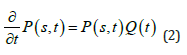
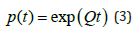
In Equation 2, Q is called the transition intensity, transition rate, or generator matrix. It is important to note that t is the time since process X(t) has started and not the time since entering the last state [15]. Therefore, the transition intensities depend on the pipe’s age and not on the duration of the last state of the wastewater. For a finite state space, computing the transition probability matrix P(t) associated with a CTMC is done using Eq.3:

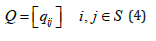
The generator matrix, Q, is defined as per Eq. 4.

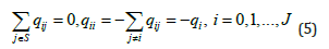
For the generator matrix, Q, the sum of all elements in a row adds up to 1, as shown in Eq.5:

The CTMC that describes the wastewater deterioration model in this study is shown in Figure 3.

Eq. 5

The matrix of transition rates Q = [q_ij] column values should be zero, and the diagonal elements are the negative sum of the offdiagonal elements in the column.

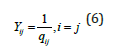
The time spent in a state before moving to the next state, the sojourn time (Y_ij), can be computed from the transition rates. As a result, the time spent in rating 1 before moving to rating 2 is calculated using the rate q₁₁, while the sojourn time in rating 2 is calculated using rate q₂₂, and similarly, the sojourn time for other ratings is calculated as shown in Eq. 6:

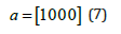
It is said that a CTMC {X(t), t ≥ 0} is fully described by its initial distribution, a, and its transition probability matrix, P(t). The initial distribution of a CTMC is a row vector representing the probability mass function of the system being in state i at time t=0 [14]. So, in the case of the CTMC presented in Figures 2-5, a is a row vector of five elements, each element representing the probability of being in any of the five states at time 0, that is, the time of installation of the pipes. Since it is assumed that the pipes were installed in perfect conditions and installed in the same year, so the initial distribution of the CTMC in this study is the row vector shown in Eq. 7:

To find the transition probabilities at any age of the wastewater pipe, the desired age must be inserted into Eq. 3. When observation data is available at age t of the pipe, transition probabilities to worse conditions at subsequent times are found from the transition probability matrix P(t+s), where s is the time elapsed from the observation (i.e., the last CCTV inspection). However, the solution’s most difficult part is finding the generator matrix because our CTMC model will only be in the present state or will move to the worst state but will not improve its condition. The major difficulty when estimating the parameters of a CTMC is that continuously observed data is not available in most cases, but only discrete-time observations exist. This is the case with wastewater condition assessment data as well. This drawback has been solved in the contributed research article of the “ctmcd” package by Pfeuffer [16] who presents several methods to estimate the generator matrix of a CTMC.

Estimation of the Generator Matrix, Q, For CTMC

The goal of this research is to use a CTMC process to model wastewater pipe deterioration, not to develop computational methods to solve for the generator matrix. There is extensive literature across various disciplines such as medicine, business, or physics that have developed a variety of computational methods for determining Q and P(t) see for example the works of [17,18]. In this work, estimation of the generator matrix, Q, was done by using the statistical software R, and implementing the “ctmcd” package [16].

The major difficulty when estimating the parameters of a CTMC is that continuously observed data is not available in most cases, but only discrete-time observations exist. This is the case of wastewater condition assessment data as well. This drawback has been solved in the contributed research article of the “ctmcd” package by Pfeuffer [16] who presents several methods to estimate the generator matrix of a CTMC. In the current research work, the Gibbs sampling method has been used, and the following paragraphs will briefly describe it. For other computational methods available in R, the reader is referred to Pfeuffer [16] and Bladt and Sørensen [17,18].

Gibbs sampling is a Monte Carlo Markov Chain (MCMC) sampling method. MCMC methods are used in Bayesian inference to characterize a distribution by randomly drawing samples out of it without knowing all of its properties [19]. Any statistic of the posterior distribution can be, theoretically, computed by simulating a large number of samples from the distribution [20]. As a note, prior and posterior distributions are used in Bayesian statistics where the prior distribution is an initial belief about the studied parameter, and it is updated based on the available data to obtain the posterior distribution of the parameter, using Bayes’ theorem.

Gibbs sampling generates posterior distributions of the parameter (or parameters) by sequentially sampling through each parameter from its conditional distribution while the rest of the parameters’ values remain fixed at their current value [20]. To have an easier understanding of this process, Yildirim [20] presented the generic algorithm of the Gibbs sampling method.

Algorithm 1 for Gibbs Sampler generalized by Yildirim

Initialize

for iteration i=1, 2,…. N do

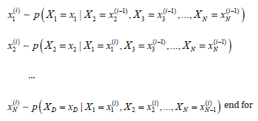
In the above generalized algorithm, the samples are generated by passing through all the conditional posterior distributions of the parameters, one random variable at a time. At the initialization, random samples are generated that might not be representative of the posterior distribution. As a result, these algorithms are typically run for many iterations and early iterations are generally discarded. The discarded samples, or iterations, are called the burn-in period [17,18,20].

To be specific, solving for the generator matrix Q in this study using the MCMC method, a prior density of the generator matrix is chosen, ϕ(Q), and the method is used to solve for the conditional distribution of Q given the existing data . Samples are drawn from the conditional distribution of (Q, X) given x, and by implementing the Gibbs sampler alternately X, is drawn given (Q, x) and Q is drawn given (X, x) by following the algorithm presented above. The continuous time sample paths of the process are represented by . Further detailed description of the Gibbs sampler is provided in Bland and Sørensen [17] with an application to estimate transition rates between credit ratings from observations at discrete points in time.

Pfeuffer [16] developed the “ctmcd” package for the R environment that allows for the implementation of the Gibbs sampling method to solve for the generator matrix of a CTMC, having only discrete observed data at times 0 and T. This is actually the case for many of the systems in the wastewater industry, where condition data is known at the time of installation (t=0, assuming an almost perfect condition), and condition inspection is performed at another time in the future at age T of the pipe. The case study presented in Section 5.5 has this type of data as well.

Bladt and Sørensen [17] proved that the Gamma distribution can be used as a prior distribution for estimating the off-diagonal elements of the generator matrix [16]. As a result, the posterior distribution is derived as shown in Eq. 8:

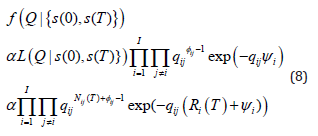
Briefly, the Gamma distribution is a two-parameter continuous probability distribution, where the first parameter, α, is called the shape parameter, and the second parameter, β, is the rate parameter. Both α and β are positive real numbers. In Eq. 8, Bladt and Sørensen [17] define a Gamma distribution with parameters ϕ and ψ: Γ(ϕ,ψ). More details about this can be found in Bladt and Sørensen [17,18].

Based on Eq. 8, the Gibbs sampler used in the “ctmcd” package samples at each iteration a full conditional distribution from the missing data, given the current parameter values and the existing observations at discrete times. The method simulates at each iteration the missing number of transitions from state i to state j and the cumulative sojourn times in each state before the process moves to another state given the current parameter estimates. New parameter values are drawn then, based on the imputed data. The sampling is run for 10,000 iterations, the first 1,000 being discarded. After the 10,000 iterations, each element of the generator matrix is sampled.

Consequence of Failure

COF model was previously built using a weightage average consisting of 5 factors related to pipe characteristics under Social Impact (SI), Economic Impact (EI), and Environmental Impact (ENVI). Therefore, a weighted rating based on the weightage average with only pipe characteristics was used to find the consequence of the failure, which means which factor requires more costs by giving them low, medium, and high values [21]. The present COF model is built on the previous COF model with 12 factors. The Hierarchical structure of the COF model is shown in Figure 4. List of factors of economic, social, and environmental factors is shown in Table 1.

Weighted average

The weighted average is a calculation considering the varying degrees of importance of the numbers in a data set. Weighted Average is calculated using Eq. 9. Weights given to the quantities can be a percentage, whole number, or decimal. The weight description is shown in Table 2.

Results

Probability of Failure:

The generator matrix using R programming shows the transition rates between conditions for the analyzed Vitrified clay (VC) pipe cohort is presented below:

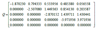
From the generator matrix, the sojourn times were calculated using Eq. 5-10. The results show that the time spent in rating 1, before moving to rating 2, is on average 29.94 years. The time spent in rating 2, before moving to rating condition 3, is 22.33 years. The time spent in rating 3, before moving to rating condition 4, is 19.51 years. The time spent in rating 4, before moving to rating condition 5, is 14.09 years. Based on the sojourn times, a VC pipe of 8-inch diameter from the analyzed cohort moves to the worst rating 5 is after 85.87 years. Figure 5 presents these results.

Once the generator matrix is found, transition probabilities for given age of pipe are easily found using Eq. 3. Note that the time interval between the observations is 56 years; therefore, a factor of (t/56) must be accounted in the exponential expression, where t is the time between the observation and desired time. The one-step transition probability matrix is therefore computed as shown below:

Thus, Equation shows the one-year transition probabilities between conditions from the last observation. The probability of failure is defined as the probability of entering the worst state that is rating 5 from any of the rating 1 is 0.001440503. The probability of failure is defined as the probability of entering the worst state that is rating 5 from any of the rating 2 is 0.004403507. The probability of failure is defined as the probability of entering the worst state that is rating 5 from any of the rating 3 is 0.025775494. The probability of failure is defined as the probability of entering the worst state that is rating 5 from any of the rating 4 is 0.068470508.

It can be verified that the sum of rows of matrix Q is 0, and the sum of rows of matrix P(1) is 1, as previously mentioned. Figure 6 shows the probability of being in any of the three states based on the pipe’s age. The plot was obtained by iterating through 200- time steps (the 200 years of life of VCP) and computing P(t) at each time step, using Eq. 3, and knowing the initial distribution, Eq. 6.

From Figure 5 the probability of being in the worst condition state of rating 5 is seen. The probability is almost 0.85 for the pipe at the age of 85 years for a comprehensive rating 5. However, it is important to note that the large data gap of 56 years is not desirable and might lead to inaccurate estimations of the generator matrix, leading to unreliable probability estimates.

Consequence of Failure:

From Figure 7, corrosion, soil type, and waste type is the main reason for pipe consequence failure. Under the economic factor, corrosion plays an essential consequence in pipe failure. Traffic loading plays an important consequence for pipe failure under social factors, and soil type and waste type play an important consequence under environmental factors. However, the developed model could not be verified because the main factors determining the consequence of failure are not mentioned in the data or the by the contractor or the inspector.

To determine a wastewater segment’s TBL COF for each wastewater, a series of factors considered under economic, social, and environmental criteria is applied to each wastewater pipe. Next, an overall COF score of the analyzed segment is calculated as a weighted average of all individual factors. This process aimed to obtain an approximate interval variability of the weighted average score based on the value. The results are summarized in Table 3 to determine the pipe’s consequence of failure. Figure 8 shows the percentage of pipes with the consequence of pipe failure ratings 1 to 5.

Conclusion

The POF model assessed the probability of pipe failure for the next 200 years. The probability is almost 0.1 for the pipe at the age of 100 years for comprehensive rating 1, which means the best condition, and the probability is almost 0.85 for the pipe at the age of 85 years for comprehensive rating 5, which means it needs immediate rehabilitation or replacement. The COF model assessed the consequences of a potential wastewater failure on a numerical scale of 1 through 5 using the TBL approach. The COF model showed Corrosion, Soil Type and Waste Type are the main consequences involving more costs of failure and 40% of pipes need moderate to high costs and 7% of pipes need high costs. The uniqueness of this work lies in incorporating many factors, precisely 12, under the economic, social, and environmental cost criteria to determine the COF score of wastewater pipes.

References

1. Report I (2021) Infrastructure Report.
2. USEPA (2004) Report to Congress: Impacts and Control of Combined Sewer Overflows and Sanitary Sewer Overflows.
3. ASCE (2021) 2021 Infrastructure Report Card.
4. Betgeri SN (2022) Analytic Hierarchy Process is not a Suitable method for the Comprehensive Rating.
5. Betgeri SN, Vadyala SR, Mattews D, John C, Lu D (2022) Wastewater Pipe Rating Model Using Natural Language Processing. arXiv preprint arXiv:2202: 13871.
6. Betgeri SN, David BS (2021) Comparison of Sewer Conditions Ratings with Repair Recommendation Reports. Proc, North American Society for Trenchless Technology (NASTT).
7. Vladeanu G, Matthews JC (2018) Analysis of risk management methods used in trenchless renewal decision making. Tunnelling and Underground Space Technology 72: 272-280.
8. Chughtai F, Zayed T (2008) Clustered Models for the Integration of Sewer Condition Classification Protocols. Pipelines 2008: Pipeline Asset Management: Maximizing Performance of our Pipeline Infrastructure, p. 1-11.
9. Baik HS, Jeong HS, and Abraham DM (2006) Estimating transition probabilities in Markov chain-based deterioration models for management of wastewater systems. Journal of water resources planning and management 132(1): 15-24.
10. Salem O, Salman B, Najafi M (2012) Culvert asset management practices and deterioration modeling." Transportation research record 2285(1): 1-7.
11. Wirahadikusumah R, Abraham D, Iseley T (2001) Challenging issues in modeling deterioration of combined sewers. Journal of infrastructure systems 7(2): 77-84.
12. Najafi M, Kulandaivel G (2005) Pipeline condition prediction using neural network models. Pipelines 2005: Optimizing Pipeline Design, Operations, and Maintenance in Today's Economy, pp. 767-781.
13. Betgeri SN, Vadyala SR, Matthews JC, Madadi M, Vladeanu G (2022) Wastewater Pipe Condition Rating Model Using K-Nearest Neighbors. arXiv preprint arXiv: 2202: 11049.
14. Kulkarni V (1995) Modeling and analysis of stochastic systems (Vol. 36). Crc Press.
15. Kallen M (2009) A comparison of statistical models for visual inspection data. Proc., Safety, Reliability and Risk of Structures, Infrastructures and Engineering Systems, Proceedings of the Tenth International Conference on Structural Safety and Reliability (ICOSSAR’2009), Citeseer, 3235-3242.
16. Pfeuffer M (2017) ctmcd: An R Package for Estimating the Parameters of a Continuous-Time Markov Chain from Discrete-Time Data. R Journal 9(2).
17. Bladt M, Sørensen M (2005) Statistical inference for discretely observed Markov jump processes. Journal of the Royal Statistical Society: Series B (Statistical Methodology) 67(3): 395-410.
18. Bladt M, Sørensen M (2009) Efficient estimation of transition rates between credit ratings from observations at discrete time points. Quantitative Finance 9(2): 147-160.
19. Van Ravenzwaaij D, Cassey P, Brown SD (2018) A simple introduction to Markov Chain Monte–Carlo sampling." Psychonomic bulletin & review 25(1): 143-154.
20. Yildirim I (2012) Bayesian inference: Gibbs sampling. Technical Note, University of Rochester.
21. Anbari MJ, Tabesh M, Roozbahani A (2017) Risk assessment model to prioritize sewer pipes inspection in wastewater collection networks. Journal of environmental management 190: 91-101.