


Time Variations of Sediment Floc Size and Density by using Settling Column Data
Hossein Samadiboroujeni1*, Sayedeh Arezoo Naghshbandi2 and Ali Altaee3
1Department of Water Engineering, Shahrekord University and visiting fellow at University of Technology Sydney, Australia
2Department of Water Engineering, Faculty of Agricultural, Shahrekord University, Iran
3Department of Civil and Environmental Engineering, University of Technology Sydney, Sydney, Australia
Submission: November 06, 2021; Published: February 22, 2021
*Corresponding Author:Hossein Samadiboroujeni, Department of Water Engineering, Shahrekord University and visiting fellow at University of Technology Sydney, Australia
How to cite this article: Hossein Samadiboroujeni, Sayedeh Arezoo N, Ali Altaee. Time Variations of Sediment Floc Size and Density by using Settling Column Data. Civil Eng Res J. 2021; 11(3): 555812. DOI: 10.19080/CERJ.2021.11.555812
Abstract
The current study was conducted to examine the sediment floc size and density changes over time in quiescent water by experimenting with a plexy glass settling column. The experiments were done with 5 initial concentrations of 3, 5, 10, 15 and 20 g/l and suspended sediment concentration was measured at different time and height intervals. Mclauglin differential equation, Kranenburg’s equation, and Stokes’ Law relationship were solved to estimate the geometrical characteristics of the flocs. In all experiments, the maximum settling velocity of particles occurred 15 minutes after the beginning of the settling process and the maximum settling velocity of sediments was obtained about 8 times the average settling velocity. The results showed that after 15 minutes of the start of the experiment, the floc size and density reached to the maximum and minimum value, respectively.
Keywords: Cohesive sediments; Floc size; Settling velocity; Settling Column
Symbols List
Introduction
The investigation of settling process and cohesive sediments consolidation in dam reservoirs and beaches is one of the most important issues playing an effective role in different descaling and sediment controlling designs, including dredging projects and hydraulic sediment removal operations. The superfine cohesive sediments even settle in the canals in which the existing standard criteria of design have been observed. They have also settled in dam reservoir and resulted in trapping efficiency near 100%. In addition to reducing the service life of reservoir, this problem has also changed the limpidity of the water released from the existing reservoir, ecology and morphology of the downstream river. In the beaches and seaports, the cohesive sediments settlement has caused an increase in dredging costs. In many cases it is impossible to overcome this phenomenon in practice [1].
A key component of fine-sediment dynamics is the settling process resulting in the deposition of sediment. Due to flocculation, the settling velocity of fine sediments is significantly more complex and dynamic than that of noncohesive sediments. Flocculation is a reversible process through which suspended fine-sediment particles are aggregated in the water column to produce flocs. Flocculation of fine sediment involves the complex interactions of particles, fluid, biology, and chemistry through the processes of aggregation, breakup, settling, and transport. Flocs are complex composite structures composed of organic (e.g., bacteria and detritus) and inorganic (e.g., clay particles) materials that are formed through attractive electrochemical forces, biochemical bonding/binding, and interparticle collisions [2].
Based on the conducted research, the settling velocity of cohesive sediments varies from 0.01 to 10 mm/s. Normally, the maximum settling velocity of cohesive sediments occurs at the concentration of 2 -10 g/l. At the higher concentrations, the flocs are broken, and their velocity decreases too [3]. Generally, the settling velocity of cohesive sediments is dependent on how sedimentary particles stock to each other, flocs formation, and their characteristics. Studies conducted by shin et al. [4] showed that floc formation is done at the first 15 minutes of cohesive sediments’ settling process, and the size of flocs reaches to its maximum value at this interval, and after that approximately remains constant until settlement occurs. This finding which is in agreement with those obtained by Spicer et al. [5] and Sanford et al. [3] shows that the maximum rate of flocculation process of cohesive sediments occurs 15 minutes after the experiment.
Zhongfan Zhu [6] developed a simple formula to relate the size and settling velocity of cohesive sediment flocs in both the viscous and inertial settling ranges. This formula maintains the same basic structure of the existing formula. However, it is amended to incorporate the fact that the flocculated sediment has internal fractal architecture and is composed of different-sized primary particles. Zhao et al. [7] developed a method to determine the settling velocity of both flocs and particles without using the fractal dimension. To achieve this goal, porosity was introduced as a substitute for the fractal dimension, and a simple method with three variables, floc diameter, mass concentration, and volume concentration of flocs, was developed. Results indicated that this method has higher accuracy than traditional methods such as the Stokes equation and the Rubey equation. Mhashhash et al. [8] used an extensive experimental setup using a particle image velocimetry (PIV) camera system to measure floc size distribution and establish a new settling velocity equation as a function of salinity and turbulence.
In practical applications involving sediment transport processes, various methods of identifying the settling velocity of flocs have been used. Numerous empirical and numerical models have been developed from laboratory and field data predicting the settling velocity of flocculated material. These models are grouped into six classes based on methods of formulation and level of complexity [9]. The six classes are listed in order of increasing complexity: (1) constant settling velocity, (2) simple empirical [10-12] (3) process-based empirical [13-16], (4) complex empirical [15,17-19], (5) fractal-based [20-22], and (6) Population Balance Equations [23,24]. It has been generalised that there are two distinct component groups of flocs: macroflocs and microflocs [18]. Macroflocs are large, highly porous (> 90%), fast settling aggregates which are typically the same size as the turbulent Kolmogorov (1941) microscale. Macroflocs( 160 m) f d > μ are recognised as the most important sub-group of flocs, as their fast-settling velocities tend to have the most influence on the mass settling flux [25]. The smaller microflow( 160 m) f d > μ are generally considered to be the building blocks from which the macroflocs are composed. Microflocs are much more resistant to a breakup by turbulent shear. Generally, they tend to have slower settling velocities, but exhibit a much wider range in effective densities than the larger macroflocs [26]. The initial research studies on the effect of sedimentary particles concentration on the settling velocity conducted by Mclauglin [27], show that the settling velocity of particles decreases as the sediment concentration increases. Researchers such as Cancio and Neves [28], Cancio and Neves [29], krone [30], Mehta and partheniades [31], and Mehta and partheniades [32] have defined the settling velocity as a function of fluid concentration. If a floc is settling within the viscous Reynolds region (i.e., when the particle Reynolds number, Re, < 0.5), the effective density for each floc could be obtained by applying a Stokes’ Law relationship:
where,μ is the dynamic viscosity of water, f ρ is the wet bulk density of floc, w ρ is the density of water, and f d is the floc diameter.
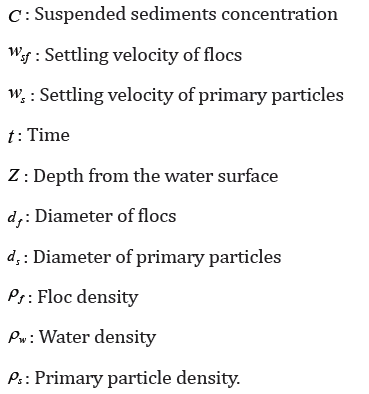
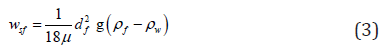
Son and Hsu, (2011) added the function of (1-φf)4 to the aforementioned equation as follows to consider hindered settling, consistent with the formula suggested by Richardson and Zaki [33]
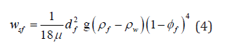
Where, f φ is the solid volume fraction which is defined as f C ρ ,C is the sediment concentration. Both f ρ and f d are variables in this equation due to the flocculation process. Kranenburg [34] developed the following relationship to estimate the floc wet bulk density f ρ:
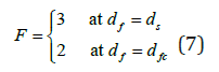
Where the densities is in g cm−3 and f d is inμm. f d is the diameter of the primary particles and F is the fractal dimension which it is not a constant but a variable ranging from around 2.0 for a large floc aggregate and approaching 3.0 when floc is disaggregated into primary particles [35]. Assumption of constant fractal dimension, if in fact, it is a decreasing function of size, would cause the observed overprediction of density and settling velocity at large and small floc sizes. It is then legitimate to consider a continuous decrease of the fractal dimension as the size of flocs increases. The following power-law represents a reasonable proposed approximation for F :

Where the coefficientα is proposed to be equal 3 and the exponentβ can be calculated using the following boundary conditions criterion [20,36,37]:
Where fc d is the characteristic floc size, this value can reach 2000μm[21].
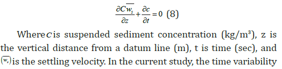
The settling velocity of the sediment is obtained from the settling column data and Mclauglin’s differential equation. Mclauglin [27] described a way for measuring the settling velocity in the quiescent water carrying solids. He established his research using settling column and the following differential equation.
Materials and Methods
Laboratory Model
In this study, to perform experiments, the settling column model was constructed in the hydraulic laboratory of Shahrekord University. The model mentioned above was made of plexy glass with a total height of 3 meter consisting of 3 pieces of plexy glass columns; each one was 1 meter in length. These pieces were connected by ring and flange. The internal diameter of the column and the plexy glass thickness was chosen to be 0.19 m and 5 mm, respectively. The lower end of the column was connected to a conelike depletion canal, and a discharge valve was embedded beneath it, and the whole model was mounted on a leggy metal chassis (Figure 1). Additionally, in order to provide a mixture of water and sediment for performing experiments, a metal reservoir with 250 L capacity equipped with electronic mixer and booster pump was made, and the water transfer pipe from the reservoir to the top of the column was embedded into the column to transfer the mixture of water and sediment. Reading the water level in the model was done using a band meter with 3m length installed on the model. To determine concentration, sampling valves were installed on the settling column at 0.2 m depth intervals for sediment sampling.

Specification of the used sediment
To conduct the current research, the sediments were collected from the dry bed of earth dam reservoir of Pirbalout located 20 km southwest of shahrekord and transferred to Laboratory. The grain size distribution curves for sediment used in this work is presented in (Figure 2). According to the gradation curve, it is found that the sediments contain 64% clay and 36% silt. The median diameter of the sediment particle, d_50, is obtained 3.5 μm. Also, the liquid limit (LL), plastic limit (PL), and plasticity index of the sediment was determined based on the ASTMD423 standard (ASTM 1972). The test showed that LL, PL, and plasticity index are 48.0, 37.2, and 10.8%, respectively. Density of the primary particles of the sediment was obtained 2.69 g/cm3.
Sediment concentration measurement
To measure the sediments concentration at different times, sediment samples (≃100cc) were collected using sampling valves and then the suspended sediment concentration was measured by drying and weighing methods. To perform these measurements, digital balance with 0.001 gr accuracy and an oven with maximum internal heat of 120°C was used.
Experiment steps
The experiments were performed in 3 steps in this research, including preparing the sediment and water mixture, transferring the mixture to the settling column model, and measuring during the settlement. In the first step, primarily the sediments were dried completely and beaten well by a metal hammer and passed through the sieve number 200. Given the initial intended concentration, a certain amount of dry sediments was selected and added to a certain amount of water in a 250 liters tank to prepare the water and sediment mixture, then using a mixer and a submersible pump (simultaneously), the mixture was completely mixed for 1 hour to ensure that no floc has formed before the settling experiment. To perform the second step, a 1 inch pump was used and the mixture of sediment and water was transferred into the model. Considering the volume of the settling column and the pump discharge, it took us 1 minute to fill the column.

The initial concentrations under the test were 3, 10, 5, 15, and 20 g/l. For each of these initial concentrations, sampling was done at different depths to determine the concentration at times of 5, 15, 30, 60, 120, 240 and 480 minutes. Samples were also taken from depths of 0.4, 0.8, 1.4, 1.8, 2.4 and 2.8 m relative to the water surface in the model. Of course, at the time of starting the experiment, a control sample was taken for each initial concentration, to estimate the initial concentration. 2-5- Settling velocity computation method. In order to estimate the settling velocity, Mclauglin equation was used, which is defined as follows.

To use the mentioned above equation, the concentration changes curve was used, and the numerator is the area under the concentration distribution curve relative to the depth at different times.
Results and Discussion
Changes in Concentration with Depth
The concentration increases by increasing depth, and as time goes by, the concentration of sediments decreases due to the sediments settlement. According to the results of measuring sediment concentration, the concentration depth distribution at different times is shown in (Figure 3, a - e). The concentration depth distribution in the conducted experiments shows that 15 minutes after the beginning of settlement, the highest gradient of depth changes in concentration occurs (on average equal to 1.25 g/l per each meter of depth). In contrast, 60 minutes after the beginning of settlement, the maximum gradient of depth changes in concentration occur (on average equal to 0.14 g/l per each meter of depth). The reason can be attributed to the flocs reaching to their maximum size after the first 15 minutes and the maximum rate of settlement at this time [3,5]. Additionally, results showed as the initial concentration of experiment increases, the gradient of deep changes in concentration increases as well, such that the average gradient of depth changes in concentration for initial concentration of 3 gr/ L is equal to 0.3 g/l per each meter of depth. And for initial concentration of 20 g/l, this gradient is equal to 0.7 g/l per each meter of depth. This may occur due to the effect of high initial concentration on increasing the settling and sedimentation rate of suspended sediments.

Changes in Concentration over Time
To investigate time changes of sediments concentration, (Figures 4 and 5) are presented. As shown in these figures, for experiments with different initial concentrations, after 15 minutes of settling, concentration changes occur gradually. Still, after this time, the concentration reduction process becomes faster, and after 60 minutes of settling, the sediment concentration reaches 12% of initial concentration. After 120 minutes, the sediment concentration reaches 5% of initial concentration. This shows that most of the sediments will be deposited in the first 1-2 hours of the experiment.
The settling velocity computation
In order to compute the settling velocity of sediments based on equation (11), at first, the numerator i.e., the surface under the


Time Variation of the Floc Diameter and Density
Under the assumption that the structure of flocs is selfsimilar, the concept of fractal geometry can be used to describe the geometrical characteristics of this structure. This concept has been applied widely to the description of floc geometry. In this work, Kranenburg’s equation and Stokes’ Law relationship have been used to estimate the time variability of the geometrical characteristics of the floc, including diameter and density. For this purpose, these two equations have been numerically solved, and the floc diameter and density were calculated at each time and level. The results of floc density calculations, as illustrated in (Figure 7), show that the floc density gets to the minimum value after 15 minutes of the start of the experiment because the flocs reach their maximum size. After reaching its minimum value, the density has an increasing trend, and it is concluded to the primary particle density. This figure also shows that the averaged floc density is decreased with the column depth. It may be because of growing the floc size with increasing the depth. The results of floc diameter calculations, as shown in (Figure 8), indicate that the floc diameter gets to the maximum value after 15 minutes of the start of the experiment because the flocs reach their maximum size. The results also show the average floc size has an increasing trend at first and after reaching its maximum value. This figure also indicates that the averaged floc size is decreased with increasing the column depth.


Conclusion
According to the findings of this study, it can be concluded that:
a. At any initial concentration, as the depth of the water column increases, the amount of concentration increases too.
b. The results show that the maximum settling velocity of sediments is about 8 times the average settling velocity of the sediments, which shows significant flocculation of the sediments.
c. The settling velocity of sediments gets to the maximum value after 15 minutes of the start of the experiment because the flocs reach their maximum size. These results are in agreement with those obtained by shin et al. [4], Sanford et al. [3] and Spiner et al. [5].
d. The results showed that the maximum amount of the settling velocity occurred at a low initial concentration of sediments (3g/l). Still, by increasing the initial concentration due to the water and sediment mixture entering into the hindered phase, the maximum amount of settling velocity of cohesive sediments began to decrease.
e. The results of floc density calculations show that the floc density gets to the minimum value after 15 minutes of the start of the experiment and after reaching to its minimum value; the density has an increasing trend. Finally, it is concluded to the primary particle density.
f. The results of floc diameter calculations indicate that the floc diameter gets to the maximum value after 15 minutes of the start of the experiment because the flocs reach their maximum size. The results also show that the average floc size has an increasing trend at first and before reaching its maximum value. The averaged floc size has also been decreased with increasing the column depth.
Acknowledgements
The authors would like to express their sincere gratitude to Shahrekord university research deputy.
References
- Samadi-Boroujeni H, Fathi-oghaddam M, Shafaie-Bajestan M, Mohammad.Vali.Saman H (2005) Modelling of Sedimentation and Self-Weight Consolidation of Cohesive Sediments, Sediment and Ecohydraulics Intercoh 2005. 1st edn, Elsevier B.V. Oxford, UK, ISBN: 978-444-53184-1 pp: 165-191.
- Mehta AJ (2014) An introduction to hydraulics of fine sediment transport. Hackensack, NJ: World Scientific pp: 1039.
- Sanford L, Dickhudt PJ, Rubiano-Gomez L, Yates M, Suttles SE (2005) Variability of suspended particle concentrations, sizes, and settling velocities in the Chesapeake Bay turbidity maximum. In: Droppo IG, Leppard GG, Liss SN, Milligan TG (eds.) Flocculation in Natural and Engineered Environment Systems. CRC Press, Washington D.C. pp: 211-356.
- Shin HJ, Son M, Lee G (2015) Stochastic Flocculation Model for Cohesive Sediment Suspended in Water. Water 7: 2527-2541.
- Spicer PT, Pratsinis SE, Raper J, Amal R, Bushell G, et al. (1998) Effect of shear schedule on particle size, density, and structure during flocculation in stirred tanks. Power Tech 97(1): 26-34.
- Zhongfan Zhu Zh (2019) A formula for the settling velocity of cohesive sediment flocs in water, Water Supply 19(5): 1422-1428.
- Zhao J, Yang G, Kreitmair M, et al. (2018) A simple method for calculating in-situ settling velocities of cohesive sediment without fractal dimensions. J. Zhejiang Univ. Sci. A 19, 544-556.
- Mhashhash A, Bockelmann-Evans B, Pan Sh (2018) A new settling velocity equation for cohesive sediment based on experimental analysis. Journal of Ecohydraulics 1-9.
- Floyd IE, Smith SJ, Scott SH, Brown GL (2016) Flocculation and settling velocity estimates for reservoir sedimentation analysis. ERDC/CHL CHETN-XIV-46. Vicksburg, MS: US Army Engineer Research and Development Center.
- Owen MW (1971) The effect of turbulence on the settling velocities of silt flocs. In Proceedings of the Fourteenth Congress of the International Association of Hydraulic Research (IAHR) 4: 27-32.
- Gibbs RJ (1985) Estuarine flocs: Their size, settling velocity and density. Journal of Geophysical Research 90(C2): 3249-3251.
- Kranck K, Milligan T (1992) Characteristics of suspended particles at an 11-hour anchor station in San Francisco Bay, California. Journal of Geophysical Research 97: 11373-11382.
- Van Leussen W (1994) Estuarine macroflocs: their role in fine-grained sediment transport, PhD thesis, Utrecht University, the Netherlands.
- Teisson C (1997) A review of cohesive sediment transport models. In Cohesive Sediments ed. Burt N, Parker R, Watts J Chichester, UK: John Wiley & Sons pp: 367-381.
- Teeter AM (2001) Clay-silt sediment modeling using multiple grain classes. Part I: Settling and deposition. In Coastal and Estuarine Fine Sediment Processes, ed McAnally WH, Mehta AJ Amsterdam, Netherlands: Elsevier Science BV pp: 157-171.
- Soulsby RL, Manning AJ, Spearman J, Whitehouse RJS (2013) Settling velocity and mass settling flux of flocculated estuarine sediments. Marine Geology 339: 1-12.
- Soulsby RL (2000) Methods for predicting suspensions of mud. HR Wallingford Report TR-104. Wallingford, Oxfordshire, UK: HR Wallingford.
- Manning AJ, Dyer KR (2007) Mass settling flux of fine sediments in Northern European estuaries: Measurements and predictions. Marine Geology 245(1-4): 107-122.
- Pejrup M, Mikkelsen OA (2010) Factors controlling the field settling velocity of cohesive sediment in estuaries. Estuarine, Coastal and Shelf Science 87(2): 177-185.
- Winterwerp JC (1998) A simple model for turbulence induced flocculation of cohesive sediment. Journal of Hydraulic Research 36(3): 309-326.
- Khelifa A, Hill PS (2006) Models for effective density and settling velocity of flocs. Journal of Hydraulic Research 44(3): 390-401.
- Strom K, Keyvani A (2011) An explicit full range settling velocity equation for mud flocs. Journal of Sedimentary Research 81: 921-934.
- Verney R, Lafite R, Brun-Cottan JC, Le Hir P (2011) Behaviour of a floc population during a tidal cycle: Laboratory experiments and numerical modeling. Continental Shelf Research 31(10) Supplement 10: S64-S83.
- Lee BJ, Toorman E, Molz F, Wang J (2011) A two-class population balance equation yielding bimodal flocculation of marine or estuarine sediments. Water Research 45(5): 2131-2145.
- Mehta AJ, Lott JW (1987) Sorting of fine sediment during deposition. Proc. Specialty Conf. Advances in Understanding Coastal Sediment Processes. Am. Soc. Civ. Eng, New York pp: 348-362.
- Fennessy MJ, Dyer KR, Huntley DA (1994a) Size and settling velocity distributions of flocs in the Tamar Estuary during a tidal cycle. Netherlands Journal of Aquatic Ecology 28: 275-282.
- Mclauglin RT (1959) Settling properties of suspensions. proc. ASCE.HY12. Paper 2311. 85: 9-41.
- Cancio L, Neves R (1995) Three-dimensional Model System for Baroclinic Estuarine Dynamics and Suspended Sediment Transport in a Mesotidal Estuary. Computational Mechanics publications 11: 353-360.
- Cancio L, Neves R (1999) Hydrodynamics and sediment suspension modelling in stuarine system. Journal of marine systems, 22: 105-116.
- Krone RB (1962) Flume studies of the transport of sediment in estuarial shoaling process Final report. Hydraulic Engineering Laboratory and Sanitary Engineering Research Laboratory, University of California, Berkeley, California p: 110.
- Mehta AJ, Partheniades E (1973) Depositional Behaviour of Cohesive Sediments. Coastal and Oceanographic Eng. Lab. Reports No.16, Univ. of Florida p: 97.
- Mehta AJ, Partheniades E (1979) Kaolinite Resuspension Properties Tech. Note. Proc ASCE 105: 164-177.
- Richardson JF, Zaki WN (1954) The sedimentation of a suspension of uniform spheres under conditions of viscous flow, Chemical Engineering Science 3: 65-73.
- Kranenburg C (1994) The fractal structure of cohesive sediment aggregates, Estuarine Coastal Shelf Sci 39(6): 451-460.
- Son, M, Hsu TJ (2011) The effects of flocculation and bed erodibility on modeling cohesive sediment resuspension, Journal of Geophysical Research 116, C03021.
- Dyer KR, Manning AJ (1999) Observation of the size, settling velocity and effective density of flocs, and their fractal dimensions. Journal of Sea Research 41(1-2): 87-95.
- Khelifa A, Hill PS (2006) Models for effective density and settling velocity of flocs. Journal of Hydraulic Research 44(3): 390-401.


