


Improving Seismic Margin Assessment Procedure using Multiple Ground Motion Parameters
Zhen Cai*, Wei-Chau Xie and Mahesh D Pandey
Department of Civil and Environmental Engineering, University of Waterloo, Canada
Submission: November 12, 2018; Published: May 15, 2018
*Corresponding author: Zhen Cai, Department of Civil and Environmental Engineering, University of Waterloo, Waterloo, Ontario, Canada N2L 3G1, Email: zhencai0821@gmail.com
How to cite this article: Zhen C, Wei-Chau X, Mahesh D P. Improving Seismic Margin Assessment Procedure using Multiple Ground Motion Parameters. Civil Eng Res J. 2018; 5(1): 555652. DOI:10.19080/CERJ.2018.05.555652
Abstract
Engineers have long recognized that "weak link” components limit the plant seismic margin, which is represented by a High Confidence of Low Probability of Failure (HCLPF) value in terms of a single ground motion parameter (GMP) such as peak ground acceleration. However, due to the use of only one GMP, inaccurate HCLPF capacities of "weak link” components are obtained, leading to unrealistic plant seismic margin.
This study proposes an improved Seismic Margin Assessment (SMA) method that overcomes the problems in traditional SMA methods, producing more realistic plant seismic margin. In particular, multiple GMPs are used to determine seismic capacities and fragilities of "weak link” components. HCLPF capacities of these components are then calculated by combining vector-valued probabilistic seismic hazard results. Numerical example of an emergency coolant injection system indicates that the proposed method would provide more realistic plant seismic margin and thus gain more reliable risk insights associated with operating nuclear power plants.
Keywords: Seismic margin assessment; Weak link components; High confidence of low probability of failure capacity; Multiple ground motion parameters; Nuclear power plant
Abbreviations: HCLPF: High Confidence of Low Probability of Failure; SMA: Seismic Margin Assessment; GMP: Ground Motion Parameter; USNRC: US Nuclear Reg-ulatory Commission; SSC: Structures, Systems, and Components; EPRI: Electric Power Research Institute; DBE: Design Basis Earthquake; RLE: Review Level Earthquake; PGA: Peak Ground Acceleration; CENA: Central and Eastern North America; NPP: Nuclear Power Plants; SSRS: Site-Specific Response Spectra; PSHA: Probabilistic Seismic Hazard Analysis; AF: Amplification Functions; UHS: Uniform Hazard Spectrum; GMRS: Ground Motion Response Spectra; ECIS: Emergency Coolant Injection System; GMP: Ground Motion Parameters
Introduction
Background
Over the past years, beyond design basis earthquake events, especially the Great Tohoku Earthquake that caused severe Fukushima Dai-ichi accident, have jeopardized the defense-in- depth concept (namely prevention, mitigation, and emergency preparedness) of traditional design philosophy. However, the traditional design methods cannot explicitly depict the plant seismic margin over the design basis earthquake. To demonstrate the plant seismic margin and to seek out "weak link” components that limit the plant seismic margin, Seismic Margin Assessment (SMA) was proposed and has been implemented in nuclear power industry since mid-1980s [1-4]. A High Confidence of Low Probability of failure capacity, namely seismic capacity related to 95% confidence of 5% probability of failure, is adopted as the measure of seismic margins of structures, systems, and components (SSCs) as well as the whole plant.
Historically, there are two methods that could be used to perform a SMA, i.e., U.S. Nuclear Reg-ulatory Commission (USNRC) SMA (described in NUREG/CR-4334) and Electric Power Research Institute (EPRI) SMA (described in EPRI-NP- 6041-SL) methods. The general procedure of both methods consists of mainly three key elements:
i. Setting screening table,
ii. Performing seismic fragility analysis, and
iii. Conducting system analysis.
The main purpose of setting screening table is to screen out SSCs whose HCLPF capacities clearly exceed the screening level so that efforts can be quickly concentrate on those SSCs for which there is a legitimate concern about seismic ruggedness. Usually, the screening level is chosen sufficiently high to demonstrate adequate plant seismic margin over the design basis earthquake (DBE). A review level earthquake (RLE) or equiv-alent seismic margin earthquake, anchored to the screening level is then defined as seismic input in seismic fragility analysis. In engineering applications, the RLE is taken as 1.67 times the DBE to indicate that the seismic risk is acceptably low. Seismic fragility analysis can be performed either by Fragility Method or by Conservative Deterministic Failure Margin method. Based on fragility analyses results, HCLPF capacities of SSCs can be calculated accordingly. Thereafter, HCLPF ca-pacities are defined as input in system analysis, which is executed either by a systematic approach making use of event trees and fault trees (implemented in USNRC SMA) or by a further simplified approach utilizing "success path" (adopted in EPRI SMA). The output is plant-level HCLPF capac-ity, representing the plant seismic margin above the DBE. Meanwhile, "weak link" components can be determined.
In engineering practice, a site-independent ground response spectrum (GRS), e.g., 5% damped NUREG/CR-0098 rock response spectrum (hereafter called NUREG spectrum) anchored to the screening level such as 0.5 G peak ground acceleration (PGA), is usually chosen as the RLE. It is well recognized that earthquake response spectra in central and eastern North America (CENA) are significantly different from NUREG spectrum, indicating that using generic GRS cannot properly capture site characteristics in the CENA. In addition, only one GMP such as PGA is used to evaluate seismic capacities and fragilities of SSCs. A fairly substantial amount of studies have shown that using only one GMP cannot predict accurate seismic responses [5,6], leading to unrealistic seismic capacities and fragilities of SSCs [7,8]. Therefore, USNRC and EPRI SMA methods would not provide accurate plant seismic margin or risk insights associated with operating nuclear power plants (NPPs).
The main purpose of this study is to propose an improved SMA method that overcomes the problems in current methods, producing more realistic plant seismic margin. In particular, an improved seismic fragility analysis method (hereafter called improved Fragility Method) is employed to determine HCLPF seismic capacities of "weak link" components. By making use of multiple GMPs, the aleatory randomness in earthquake response spectra are properly captured and seismic capacities are more accurately characterized. Therefore, more accurate HCLPF capacities of "weak link" components are obtained, bringing out more realistic plant seismic margin estimate. Another motive of this study is to help reactor licensees make more rational decision on whether modifications and improvements should be made.
Literature
With the increasing knowledge from seismological, geological, and geotechnical investigations, performance-based site-specific response spectra (SSRS) have been recommended to design nu-clear facilities [9,10]. The development of SSRS incudes four key steps:
A. performing probabilistic seismic hazard analysis (PSHA) to determine seismic hazard curves at the hard rock and the controlling earthquake,
B. conducting dynamic site response anal-ysis to calculate site amplification functions (AFs),
C. determining the uniform hazard spectrum (UHS) at the ground surface by convolving seismic hazard curves at the hard rock and the AFs, and
D. multiplying the UHS at the ground surface by a scale factor to obtain the SSRS that satisfy a target performance goal.
Regulatory Guide 1.208 [11] adopted this performance- based design procedure to develop site-specific Ground Motion Response Spectra (GMRS), namely free-field horizontal and vertical ground motion response spectra at the plant site. Thereafter, NUREG-0800 [12] required that the GMRS should be used to determine the adequacy of Certified Seismic Design Response Spectra.
Following the Fukushima Dai-ichi accident in March 2011, USNRC [13] issued a letter entitled "Request for Information Pursuant to Title 10 of the Code of Federal Regulations 50.54(f) Regarding Recommendations 2.1, 2.3, and 9.3, of the NearTerm Task Force Review of Insights from the Fukushima Dai- ichi Accident" (hereafter called 50.54(f) letter). The 50.54(f) letter required reactor licensees to perform seismic hazard reevaluations and walkdowns, and thus determined if reactor licenses should be modified, suspended, or revoked. EPRI SMA is unacceptable for satisfying the requirements of the 50.54(f) letter because it uses "success path" in system analysis.
In response to the 50.54(f) letter, USNRC [14] provided several enhancements for performing the USNRC SMA associated with the existing NPPs (hereafter called the enhanced USNRC SMA). In particular, spectral shape of the RLE should take the envelop of the DBE and the GMRS, taking into account the site-specific effects. Thereafter, EPRI [15] provided an acceptable approach for performing the SMA that satisfies the seismic elements of the 50.54(f) letter. In this approach, seismic Probabilistic Risk Assessment (PRA) may be performed to evaluate seismic risk and main risk contributors.
In 2009, USNRC issued an interim staff guidance on PRA- based SMA for new reactors, supple-menting the guidance NUREG-0800 [13] and DC/C0L-ISG-03 [16] that incorporate the PRA information into the review of NPPs. Comparing to the EPRI and USNRC SMA, the PRA-based SMA addressed the site-specific effects such as seismically induced lique-faction and foundation failure in the determination of plant-level HCLPF capacity. A screening table with screening level 1.67 times the site- specific GMRS is set to screen out SSCs whose HCLPF capacities clearly exceed the screening level. Seismic fragility evaluation is performed based on the site-specific GMRS, taking into account the site-specific effects. HCLPF Max/Min method (i.e., for components in parallel connection, the maximum HCLPF is taken, whereas for components in serial connection, the minimal HCLPF is taken) is acceptable for calculating plant-level HCLPF capacity. The plant seismic margin should be demonstrated to be equal or higher than 1.67 times the GMRS, indicating that the seismic risk is acceptably low.
Limitations of literature
A lot of literature have emphasized the importance of considering site-specific effects in the SMA. However, a number of problems have not jet been resolved in the enhanced USNRC SMA or the PSA-based SMA:
a. In the literature, scalar PSHA is performed to determine the UHS at the ground surface. The GMRS is then determined by multiplying the UHS by a scale factor. Cai [17] found that the UHS implies that spectral accelerations at any two frequencies are perfectly correlated, which contradicts with empirical correlation results. Based on this assumption, seismic responses of SSCs are overestimated [18], and the aleatory randomness in earthquake response spectra is improperly treated [7].
b. The literature used only one GMP (e.g., PGA) for performing seismic fragility analysis, neglecting the influence of spectral accelerations at dominant modes of SSCs on seismic capacity and fragility estimates. Recent studies [7,8] have shown that this influence is noticeable and should be taken into consideration. In particular, spectral accelerations at dominant modes of "weak link” SSCs should be chosen as GMPs in seismic fragility analysis.
c. The literature used a fixed spectral shape of the RLE in seismic fragility analysis, neglecting ground motion intensity effect on input GRS. Many studies [7,9] have shown that spectral shapes depend on earthquake ground motion levels, so this effect should be taken into consideration.
Objectives and organizations
This central objective of this study is to propose a SMA method that improves the enhanced USNRC SMA and the PRA-based SMA, producing more realistic plant seismic margin estimate. To achieve this objective, HCLPF capacities of "weak link” components are determined by the improved Fragility Method, whereas HCLPF capacities of less important components are calculated in accordance with the traditional Fragility Method. This ensures that more accurate plant seismic margin is achieved while the computational cost is acceptable.
This study is organized as follows. Section 2 presents a general procedure of the proposed SMA method. The key element of the procedure, namely the improved Fragility Method, is briefly introduced. Numerical example of an emergency coolant injection system (ECIS) is performed in Section 3. The enhanced USNRC SMA is conducted first to evaluate the seismic margin of the ECIS. It is found that the ECIS cannot meet the seismic requirements of the 50.54(f) letter. However, when the improved Fragility Method is employed for determining HCLPF capacity of the "weak link” component, the ECIS finally satisfies seismic requirements. The last Section 4 summarizes the key elements and demonstrates the main contributions of the study
Improved Seismic Margin Assessment
The improved SMA method is based upon the enhanced USNRC SMA (for existing NPPs) and the PRA-based SMA (for new NPPs) methods. Its purpose is not to take the place of these two methods, but is to improve these two methods by employing the improved Fragility Method to calculate HCLPF capacities of "weak link” SSCs.
Procedure
The general procedure of the proposed SMA method is presented as follows:
I. Perform the enhanced USNRC SMA (for existing NPPs) or the PRA-based SMA (for new NPPs) to evaluate plant seismic margin and to find out "weak link” SSCs
II. Consider two cases based on seismic margin results in Step 1
a) Plant seismic margin satisfies the seismic elements of the 50.54(f) letter (for existing NPPs) or of DC/COL- ISG-020 (for new NPPs).
No more efforts would be made because adequate seismic margin is demonstrated.
b) Plant seismic margin cannot meet seismic requirements
Calculate HCLPF capacities of "weak link” SSCs by employing the improved Fragility Method. If their HCLPF capacities exceed the screening level, plant seismic margin would eventually meet seismic requirements; otherwise, further efforts (e.g., seismic PRA) need to be made to demonstrate the plant seismic risk is acceptably low.
By making use of multiple GMPs in the improved Fragility Method, conservatism included in the enhanced USNRC SMA and the PRA-based SMA are effectively removed. Therefore, higher plant seismic margin estimate is expected. For existing and new NPPs that cannot satisfy the seismic margin requirements, the proposed method is undoubtedly a valuable choice, because it may avoid computationally expensive seismic PRA that aims to demonstrate acceptably low plant seismic risk.
Improved fragility method
The improved Fragility Method plays a key role in the proposed SMA method. It includes mainly three key components:
i. Seismic fragility analysis considering multiple GMPs,
ii. Vector-valued probabilistic seismic hazard analysis, and
iii. Determination of seismic fragility curves and HCLPF capacity. Based upon more accurate seismic hazard and
seismic capacity estimates, the method produces more accurate weighting (as opposed to the traditional) seismic fragility curves and HCLPF capacities. In the following, three key components are presented.
Seismic fragility analysis considering multiple GMPs:
Definition: For clarity of exposition of this section, the method is described for the two-dimensional case, i.e., two ground motion parameters (GMPs). The seismic fragility of a structure is expressed as the probability of failure, i.e., structural capacity (such as tensile strength) is less than its seismic demand (such as tension stress), conditional on a ground motion characterized by spectral accelerations SA(f) and sa/) at its natural frequencies:

Where C is the structural capacity and D is the seismic demand. s and s are spectral values of two GMPs from an earthquake response spectrum at the site. Note that Pf denotes not cumulative probability but conditional probability of failure.
A traditionally used assumption, namely basic variables in response and capacity are lognor-mally distributed [19], is adopted as well in this method. Structural capacity C and seismic demand D are therefore lognormally distributed due to multiplication of lognormal random variables.
Response spectra method is employed to calculate structural responses of important SSCs. Given an earthquake response spectrum, only spectral accelerations at natural frequencies are used in the calculation. A smooth ground response spectrum (GRS) with spectral values sl and s2 is therefore used to represent the earthquake response spectrum at the site. To cover all combinations of spectral values of two GMPs in twodimensional spectral domain, a large amount of GRS with various combinations are defined as seismic inputs in structural response analyses.
For simplicity of presentation, the condition of given ”SA/ = VSA(f2) = s2” is dropped; hence equation (1) can be rewritten as

Determination of seismic fragility: An intermediate random variable, termed as ratio factor R, is used to calculate fragility parameters. Given an input GRS with spectral values s(l) and s2'2) (hereafter abbreviated as s(') ) of two GMPs, r(s0)) is defined as the ratio of structural capacity to its seismic demand, i.e.,

Where Rm(s°)) is median ratio factor. The random variables %(s<0) and %(s<0) are lognormally distributed with unit median (zero logarithmic mean) and logarithmic standard deviations of β (s0) and βU(s'0), respectively.
In terms of the ratio factor, probability of failure of a structure conditional on s(i)is can be rewritten as

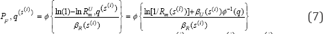
Due to lack of knowledge, the estimated median ratio factor RmU(s(i))=Rm(s(i))εU(s(i)) in equation (3) is log normally distributed, namelyRmU(s(i))=Rm(s(i))εU(s(i)). Note that εU(s(i)) is log normally distributed with logarithmic median of zero and logarithmic standard deviation εU(s(i)) i.e., εU∼LN(0,ε2(s(i)) given a confidence level Q=q, based on probability theory, εU∼LN(0,ε2(s(i)) is expressed as
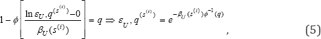
Where ø(.) denotes cumulative probability of a univariate standard normal variable. ()()UimRs at Q=q is thus determined by

Finally, as in equation [2.3], R(s ) at Q=q is lognormally distributed with parameters RUm (s<0) P (s(i)) εU∼LN(0,ε2(s(i)), q(s ), p*(s(‘}). Seismic fragility of the structure is therefore calculated by solving equation [4]:
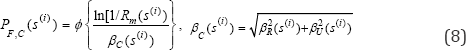
When composite variability % (s <0) = % (s <))£U (s <0) is used, R (s(0) is lognormally distributed, i.e., R(s<0)~ ln (in r (s<0), p2
Vector-valued probabilistic seismic hazard analysis: Based on vector-valued probabilistic seismic hazard analysis (PSHA), the annual rate density of {sa(/2)|sa(,;i)-si} is given by [17]
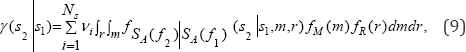
where N is the total number of surrounding seismic sources, v s the annual rate of occurrence of earthquakes with magnitude greater than a lower bound threshold value mmin (e.g., mmin = 5.0) of seismic source i. fsA / )|sa / )(s2si,mr) is the probabilistic density function PDF) of {sa(f2)|sa(f1 )-s1} conditional on an earthquake with earthquake magnitude m, and source-to-site distance r. fM (m) and fR (r) are the PDFs of m and r, respectively
The PDF of {sa(/2)|sa(/1)-s1} is then given by

The annual rate of events at the site with Sa (/ 2) between y1 and y2 conditional on sa (f2 ) = s1 is thus calculated by

For an input GRS with spectral value s of sa(f), the probability of SA (f2) being between y1 and y2, termed as "weight", is finally given by
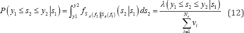
Having obtained p(y, ≤ s2 ≤ y2 |s,), the aleatory randomness in SA(/2) for a given spectral value of SAf can be properly evaluated.
Development of weighting seismic fragility curves: By applying total probability theorem with one conditional variable, given a confidence level Q = q, weighting (as opposed to traditional) seismic fragility in terms of SA / is expressed as

Numerical method is used to quantify the integral, i.e.,

Where pf,(s2(i 2) = si) is calculated by equation (7), and p(s2('21
Changing value s of sa(/) from lower bound value (e.g., 0.05G ) to upper bound value (e.g., 5G ), would give weighting seismic fragility curves at confidence level Q = Q. In practice, confidence level Q is usually taken as discrete values, such as 5%, 50%, and 95%. Therefore, seismic fragilities of the structure are represented by a family of weighting seismic fragility curves.
When composite variability is used, the composite (mean) weighting seismic fragility in terms of SA (/1) is quantified by

Where pf,c(s2('2’,s,) is calculated by equation (8). Instead of a family of weighting seismic fragility curves, a composite weighting seismic fragility curve could be used to represent seismic fragility of the structure.
To determine the HCLPF capacity, weighting seismic fragility curve at confidence level Q = 95% is used. Taking weighting seismic fragility Pf q = 5%, one can easily find weighting HCLPF seismic capacity (iHCLPF) from this curve, in which £ denotes weighting capacity.
Numerical Example - Emergency Coolant Injection System
In CANDU reactors, the emergency coolant injection system (ECIS) protects the fuel and heat transport system boundary when normal cooling fails. Its purpose is to refill the heat transport system after a loss of coolant accident and keep it full. This sets up an alternative heat flow path for removing decay heat. Following the failure of the ECIS, a core damage accident might occur. In this section, seismic margin of an example of simplified ECIS is determined for demonstrating the advantages of the proposed SMA method. A fault tree associated with the ECIS is developed to consider all possible faults. The accident sequence following the initiating seismic event (i.e., failure of the ECIS) would not be developed, because this example does not aim to evaluate the sequence-level HCLPF capacity.
Probabilistic Seismic hazard analysis
Suppose that the ECIS is used in the CANDU reactor building of Darlington nuclear generating station (NGS). The Darlington NGS (43.53° N, 78.43° W) is located on the north shore of Lake Ontario, Region of Durham in Ontario, Canada. The map information around Darlington NGS site is shown in Figure 1.

Cai et al. [8] have performed the PSHA for the Darlington NGS site. The results are seismic hazard curves with respect to specified GMPs, respectively. Figure 2 gives mean seismic hazard curves for spectral accelerations at nine representative frequencies, e.g., 0.2, 0.5, 1, 2, 3.33, 5, 10, 20, and 50 Hz. A mean uniform hazard spectrum (UHS) regarding a specific seismic hazard, i.e., mean annual frequency of exceedance (MAFE) value, can be determined based on these hazard curves. Figure 3 gives site-specific mean UHS at MAFE of 1*10-4.

The GMRS can be developed according to Regulatory Guide 1.208 [12]. The slope factor ARs with respect to a frequency is determined by

Based upon seismic hazard curves in Figure 2, AR regarding representative frequencies are calcu-lated and listed in Table 1. The design factor (DF) is then calculated by

The DFs are presented in Table 1. Due to large uncertainty in the PSHA model, DFs are significantly greater than 1. Finally, the GMRS can be determined by multiplying the UHS by DFs, and is shown in Figure 3.

According to the 50.54(f) letter, the plant seismic margin should be equal or higher than 1.67 times the GMRS to demonstrate that the seismic risk is acceptably low. Based on the site-specific GMRS in Figure 3, SA (F=50Hz) is equal to 0. 34G. It is well recognized that, for plant sites in the central and eastern North America (Darlington NGS site is within this region), spectral accelerations attenuate to PGA at around 100Hz. Therefore, the PGA value should be lower than 0.34G. In this example, PGA regarding the GMRS is taken as 0.3G based on rational judgement. The screening level is thus chosen as 0. 3*1.67=0.5G PGA. Thereafter, 1.67 times the GMRS is taken as the Review Level Earthquake (RLE) and is shown in Figure 3.

Emergency coolant injection system
Basic configuration: A simplified ECIS is shown in Figure 4. The system consists of a water tank T, a manual valve V that is normally open, two pumps P1 and P2, two check valves CV1 and CV2, and three motor-operated valves MV1, MV2, and MV3 that are normally closed. When the ECIS is activated, the injection signal is delivered to operate pumps P1 and P2, and to open the motor-operated valves MV1, MV2, and MV3. The success criterion is that water flow is delivered from at least one pump through at least one motor-operated valve.

Fault tree: The ECIS can be divided into three subsystems: Suction Line, Pump Systems, and Injection Lines, as shown in Figure 4. The Suction Line consists of the Water Tank and the manual valve V. It fails when the tank fails (no water supply) or the manual valves fails (not able to remain open). The Pump Segments subsystem has two flow routes PS-A and PS-B connected in parallel. Each flow route consists of a pump and a check valve connected in series, which fails if no signal is delivered to operate the pump, or the pump fails to operate, or the check valve is not open. This subsystem fails when both flow routes fail. The Injection Lines subsystem consists of three motor-operated valves connected in parallel, which fails when all three injection lines fail. An injection line fails if no signal is delivered or the valve fails to open. The Emergency Coolant Injection (ECI) Signal control in assumed to located in an electric cabinet. The ECI Signal fails to deliver if the cabinet falls down due to anchorage failure.
Define the following events:
E= ECIS fails (ECIS fails to deliver at least one pump of flow),
S= No ECI Signal delivered (electric cabinet falls down).
The fault tree of the ECIS as shown in Figure 5.

Seismic margin: For the ECIS, failures of water tank, pump, and electric cabinet are assumed to be governed by anchorage failure, while manual valve, check valve, and motor-operated valve (MOV) are assumed to be controlled by functional failure during the earthquake. The main aim of this example is to demonstrate the advantages of the improved SMA method, so postulated fragility parameters of components are used. Given these fragility parameters, HCLPF seismic capacities can be calculated by the traditional Fragility Method and are presented in Table 2. The electric cabinet is identified as "weak link" component.

Based upon the fault tree in Figure 5, HCLPF Max/Min method is used to evaluate the HCLPF of the ECIS. Because the electric cabinet and other events (including basic faults and sub-events) are in serial connection, the HCLPF capacity of the ECIS is equal to the minimal HCLPF value, namely 0.4G PGA. Recall that the seismic margin should be equal or greater than 0.5G PGA in accordance with the 50.54(f ) letter; thus the ECIS cannot meet the seismic margin requirement.
Seismic margin of the electric cabinet: In this section, the improved Fragility Method is used to determine more accurate HCLPF capacity of the cabinet. Based on this HCLPF capacity, engineers would make more rational decision on whether further efforts should be done.
Details of the cabinet is shown in Figure 6 and properties are listed in Table 3 [20]. It has a height H, width B, and length L of 96 inches, 30 inches and 48 inches, respectively. It is anchored by four 0.5 inch diameter WEJ-IT expansion bolts as shown in Figure 6. The base of the cabinet has a strong, stiff frame through which the bolts are attached near each corner of the cabinet so that the anchorage capacity is controlled by the bolts and not by the cabinet base. The concrete floor on which the cabinet locates contains an 18-inch by 36-inch cutout for passage of electrical cables into the cabinet. The cabinet is estimated to weight about 2500 pounds (2.5kip) and is located at the ground floor of the reactor building. The cabinet center of gravity is estimated to be at mid-height (48 inches above the base).


The electric cabinet is subjected to earthquake excitations from three directions. The funda-mental frequencies of the electric cabinet in two horizontal directions are both estimated to be =8Hz. Since the cabinet is seismically robust in vertical direction, fundamental frequency in this direction is taken as =50Hz. In the following, the HCLPF capacity of the cabinet is calculated in accordance with the improved Fragility Method.
Weights of input GRS: Since the fundamental frequencies of the cabinet in two horizontal directions are both equal to Fh =8Hz, two GMPs, i.e., SA (Fh) and PGA, are chosen as GMPs. Vector-valued PSHA is performed to calculate mean annual rate density of SA (Fh ) PGA at varying PGA values. Figure 7 gives mean annual rate density of SA (Fh ) PGA at three PGA values. Given a PGA value, the weights of input GRS with spectral values of SA (Fh ) are determined by equation (12). Changing the spectral value of SA (Fh ) from 0.1G to 5G, the weights for all input GRS given the PGA value can be obtained. Thereafter, changing PGA from 0.05G to 2.5G and repeating the procedure would result in a two-dimensional distribution of weights as shown in Figure 8.


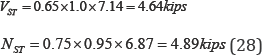
Seismic fragility analysis considering multiple GMPs:Since two GMPs are used, a great number of input GRS are needed to be defined as input GRS. In the following, conditional probability of failure of the cabinet given an input GRS (thick black line in Figure 9), is calculated for example. The vertical input GRS can be obtained using V/H ratios in the PSHA report by AMEC [21]. For FV =50Hz, one can obtain V / H =0.865; Hence, spec-tral acceleration in vertical direction s (F) =0.6x0.865=0.52G. Table 4 summarizes spectral accelerations at frequencies in three directions.


Median seismic demand in H1 direction: In the H1 direction , under seismic excitation, the tank is subjected to an inertia force equal to the product of its weight W and the spectral acceleration aH .8G, as shown in Figure 6. The inertia force is then transferred to the supports, exerting tension and shear force on anchor bolts. Assume that all anchor bolts are in elastic tension and shear during earthquake excitations. The geometric information of the cabinet is given in Table 3.
Shear force is induced in all the anchor bolts in all the supports evenly. For a single bolt, the shear force is

Tension forces in the support are due to the moment w aH .Hcg , as shown in Figure 10. For the critical anchor bolts, the tension force is given by

Median seismuic demand in vertical direction: In the vertical direction, under seismic excitation, the inertial force of the tank due to vertical acceleration aV =0.52G is transferred to the support as pure tension force, without shear force. All anchor bolts share the seismic load evenly so that the tension force is


The moment induces tension forces in the anchor bolts at 2 locations, as shown in Figure 10. For the critical anchor bolts, the tension is

Median demand in vertical direction: In the vertical direction, under seismic excitation, the inertial force of the tank due to vertical acceleration aV =0.52G is transferred to the support as pure tension force, without shear force. All anchor bolts share the seismic load evenly so that the tension force is

When the bolts are in tension, the dead load of the electric cabinet also exerts forces in the anchor bolts. All the bolts share the dead load evenly as

Combination of seismic demand from three directions: 100-40-40 percent combination rule is used to combine the maximum responses from the three earthquake components calculated separately [22]. To combine the effect of the three earthquake components on the critical anchor bolt, first assuming that the H1 direction controls and then assuming that the H2 direction controls. It is obvious that the vertical direction will not control; thus this case is not considered further.
i. H1 direction controls:
Tension force in the critical anchor bolt is:
NH1=NH1+0.4NH2+0.4NHF
=1.0 X 1.846+0.4X1.091+0.4X0.324=2.412kips
Shear force in the critical anchor bolt is

ii. H2 direction controls:
Tension force in the critical anchor bolt is:
NH2=NH2+0.4H1+0.4NHV
=1.0 X 1.091+0.4X1.846+0.4X0.324=1.959kips
Shear force in the critical anchor bolt is

The tension and shear demand of the electric cabinet are summarized in Table 5. It is easily to find that the H1 direction is the controlling direction.

Structural capacity analysis: It is assumed that the cabinet itself was designed to be seismically robust. As stated in this section, anchorage capacity is controlled by the bolts and not by the cabinet base. According to EPRI-NP-6041-SL [3] and ACI 349-06 [23], median shear and tension capacities of an anchor bolt are obtained as
Median ratio factor: Since anchor bolts are subjected to tension and shear simultaneously, a tension-shear interaction relationship, as shown in Figure 11, is used.

To determine the median strength factor, two regions in Figure 11, To determine the median strength factor given the input GRS, two regions, i.e., pure tension region and shear/ tension region are considered.
The median strength factor is given by

ii. Shear/Tension region
The median strength factor is given by
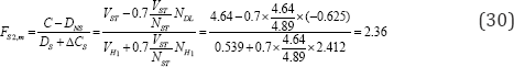
The controlling failure mode is pure tension failure of the critical anchor bolt in H1 direction.
In this study, foundation-structure interaction effect is not considered. The variabilities in damping, modelling, modal combination, and earthquake component combination are assumed to be lognormal with unit median (zero logarithmic mean) values. For the anchor bolts, horizontal peak response is unit median (Table 3) [20]. Because response spectra method is used to calculate seismic responses of the cabinet, there is no time history simulation variability. Therefore, median response factor FRSm is equal to 1.0.
Having obtained FS,m and FRS,m, and neglecting inelastic energy absorption effects, i.e., f = 1.0, median ratio factor Rm can be determined by

Logarithmic standard deviations: The approximate second-moment procedure is applied to calculate variability of ratio factor R due to basic variables. The variability from basic variables are enumerated in Table 6.

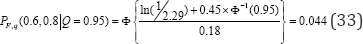
Determination of seismic fragility: Having obtained median ratio factor r- and logarithmic standard deviations pR and pJ, given the input GRS, conditional probability of failure Pf,q 0.6, 0.8 , at confidence level Q = Q, can be
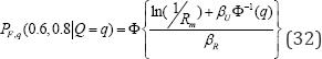
Taking confidence level Q = 95% for example, PF.A(0.6,0.8Q=0.95) is given by
Development of seismic fragility surfaces: Defining input GRS with spectral acceleration values at three frequencies from other combinations, and repeating the procedure for calculating conditional probability of failure values result in a family of seismic fragility surfaces, as shown in Figure 12 [24].


Development of weighting seismic fragility curves:
Having obtained the weights of input GRS and seismic fragility surfaces, the weighting seismic fragility in terms of PGA, at confidence level Q = q is determined by
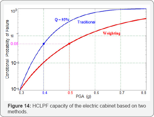
Changing PGA values from lower bound of 0.05 G to upper bound of 2.5 G results in weighting seismic fragility curves, as shown in Figure 13.

Comparison of seismic margin results
The seismic fragility curves by the traditional Fragility Method are plotted together with the weighting curves. It shows that the weighting median seismic capacity of the cabinet has 66.67% increase, i.e., from 1.14 G PGA to 1.90 G PGA. In addition, HCLPF seismic capacity of the cabinet, as shown in Figure 14, has 25% increase (from 0.4 G PGA to 0.5 G PGA). Both results indicate that the improved Fragility Method effectively digs out the conservatism in the traditional method and thus obtains more accurate median and HCLPF capacity of the cabinet [25].
Based on HCLPF Max/Min method, the HCLPF capacity of the ECIS is equal to the minimal HCLPF value in the serial connection, namely 0.5 G PGA. Therefore, the ECIS actually satisfies seismic requirements of the 50.54(f) letter. The results indicate that, for existing NPPs that cannot satisfy the seismic margin requirements, the improved SMA should be performed to reevaluate HCLPF capacities of the "weak link" SSCs. More realistic plant seismic margins would be obtained and thus more rational decision would be made.
Summary
In recent years, the enhanced USNRC SMA and the PRA-based SMA were proposed, taking into account up-to-date seismic safety requirements. In particular, the site-specific Ground Motion Response Spectra are used to demonstrate adequate seismic margin associated with operating NPPs. However, due to the use of a single ground motion parameter (GMP), conservative High Confidence of Low Probability of Failure (HCLPF) capacities of structures, systems, and components (SSCs) are obtained, leading to underestimation of plant seismic margin [26].
This study proposed an improved SMA procedure that overcomes the disadvantages of the current SMA methods, producing more realistic plant seismic margin estimates. In particular, the improved Fragility Method is used to calculate HCLPF capacities of "weak link" SSCs. Because the conservatism included are effectively removed, higher HCLPF capacities of these components are obtained. It is well recognized that, "weak link" SSCs limit plant seismic margin. Based on higher HCLPF capacities of "weak link" SSCs, greater plant seismic margin would be determined. For those NPPs that cannot satisfy the seismic elements of the 50.54(f) letter (for existing NPPs) or of DC/C0L-ISG-020 (for new NPPs), the proposed method should be implemented to reevaluate their seismic margins.
Numerical example for an emergency coolant injection system (ECIS) is performed to demon-strate the advantages of the proposed method. The results show that, by performing the improved Fragility Method, HCLPF capacity of the "weak link" component, i.e., electric cabinet, has a notice-able 25% increase, namely from 0.4 G PGA to 0.5 G PGA. The seismic margin of the ECIS thus meets seismic requirement of the 50.54(f) letter. It indicates that the proposed method can effectively increase plant seismic margin estimate, and thus may avoid computationally expensive seismic PRA [27-29].
The proposed SMA method has four major contributions as follows:
i. Use multiple GMPs to determine seismic capacities and fragilities of SSCs
ii. Perform vector-valued PSHA to capture the aleatory randomness in earthquake response spectra and to consider ground motion intensity effect on the input GRS
iii. Employe the improved Fragility Method to evaluate HCLPF capacities of "weak link" SSCs
iv. Propose an applicable and cost-effective SMA procedure.
In summary, the proposed MA method takes the advantages of the current SMA methods and the improved Fragility Method, producing more realistic plant seismic margin estimate. It should be implemented in nuclear power industry for determining more realistic seismic margins and gaining more rational risk insights associated with operating NPPs.
Acknowledgment
The research for this paper was supported, in part, by the Natural Sciences and Engineering Research Council of Canada (NSERC) and University Network of Excellence in Nuclear Engineering (UNENE).
References
- Budnitz RJ, Amico PJ, Cornell CK, Hall WJ, Kennedy RP (1985) An Approach to the Quantification of Seismic Margins in Nuclear Power Plants, NUREG/CR-4334. U.S. Nuclear Regulatory Commission.
- Kennedy RP, Campbell RD, Cassawara RP (1988) A Seismic Margin Assessment Procedure. Nuclear Engineering and Design 107: 61-75.
- EPRI (1991) A Methodology for Assessment of Nuclear Power Plant Seismic Margin (Revision 1), EPRI-TR-103959. Electricity Power Research Institute.
- Ravindra MK (1997) Seismic Individual Plant Examination of External Events of US Nuclear Power Plants: Insights and Implications. Nuclear Engineering and Design 175: 227-236.
- Bazzurro P (2002) Vector-valued Probabilistic Seismic Hazard Analysis. Proceedings of 7th US. National Conference on Earthquake Engineering, Boston, Massachusetts.
- Baker JW, Cornell CA (2005) A Vector-valued Ground Motion Intensity Measure Consisting of Spectral Acceleration and Epsilon. Earthquake Engineering and Structural Dynamics 34: 1193-1217.
- Cai Z, Xie WC, Pandey MD, Ni S (2017) Determining Seismic Fragilities of Structures and Components in Nuclear Power Plants Using Multiple Ground Motion Parameters: Part I: Methodology (in review). Nuclear Engineering and Design.
- Cai Z, Xie WC, Pandey MD, Ni S (2017) Determining Seismic Fragilities of Structures and Components in Nuclear Power Plants Using Multiple Ground Motion Parameters: Part II: Application (in review). Nuclear Engineering and Design.
- McGuire MK, Silva WJ, Costantino CJ (2001) Technical Basis for Revision of Regulatory Guidance on Design Ground Motions: Hazard- and Risk- Consistent Ground Motion Spectra Guidlines. NUREG/CR- 6728. US Nuclear Regulatory Commission.
- ASCE (2005) Seismic Design Criteria for Structures, Systems, and Components in Nuclear Power Plants, ASCE 43-05. American Society of Civil Engineers.
- USNRC (2007) Standard Review Plan for the Review of Safety Analysis Reports for Nuclear Power Plants, NUREG-0800. US Nuclear Regulatory Commission.
- USNRC (2007) A Performance-based Approach to Define the Site- specifc Earthquake Ground Mo-tion, Regulatory Guide 1.208. US Nuclear Regulatory Commission.
- USNRC (2012) Request for Information Pursuant to Title 10 of the Code of Federal Regulations 50.54(f) Regarding Recommendations 2.1, 2.3, and 9.3, of the Near-term Task Force Review of Insights from the Fukushima Daiichi Accident, DC/C0L-ISG-2012-04. U.S. Nuclear Regulatory Commission.
- USNRC (2012) Guidance on Performing a Seismic Margin Assessment in Response to the March 2012 Request for Information Letter, DC/ C0L-ISG-2012-04. US Nuclear Regulatory Commission.
- EPRI (2013) Seismic Evaluation Guidance: Screening, Prioritization and Implementation Details (SPID) for the Resolution of Fukushima Near-Term Task Force Recommendation 2.1: Seismic, EPRI 1025287. Electricity Power Research Institute.
- USNRC (2008) Interim Staff Guidance Probabilistic Risk Assessment Information to Support Design Certification and Combined License Applications, DC/C0L-ISG-03. U.S. Nuclear Regulatory Commission.
- Cai Z (2017) Seismic Fragility Analysis for Structures, Systems, and Components in Nuclear Power Plants. Doctoral Dissertation, University of Waterloo, Waterloo, ON.
- Baker JW (2011) Conditional Mean Spectrum: Tool for Ground Motion Selection. Journal of Structural Engineering 137 (3): 322-331.
- Kennedy RP, Ravindra MK (1984) Seismic Fragilities for Nuclear Power Plant Studies. Nuclear Engineering and Design 79(1): 47-68.
- EPRI (1994) Methodology for Developing Seismic Fragilities, EPRI- TR-103959. Electricity Power Research Institute.
- AMEC (2009) Site Evaluation of the OPG New Nuclear at Darlington: Probabilistic Seismic Hazard Assessment. AMEC Geomatrix, Toronto.
- USNRC (2006) Combining Modal Responses and Spatial Components in Seismic Response Analysis, USNRC R.G. 1.92. US Nuclear Regulatory Commission.
- ACI (2007) Code Requirements for Nuclear Safety-Related Concrete Structures and Commentary, ACI 349-06. American Concrete Institute.
- ASCE/ANS (2009) ASME/ANS RA-S Standard for Level 1/ Large Early Release Frequency PRA for NPP Applications. American Society of Mechanical Engineers/ American Nuclear Society.
- CSA (2010) Design Procedures for Seismic Qualification of Nuclear Power Plants, CSA N289.3-10. Canadian Standard Association.
- EPRI (2011) Advanced Methods for Determination of Seismic Fragilities: Seismic Fragilities Using Scenario Earthquakes, EPRI 1022995. Electricity Power Research Institute.
- Kennedy RP (2011) Performance-goal Based (Risk Informed) Approach for Establishing the SSE Site- specific Response Spectrum for Future Nuclear Power Plants. Nuclear Engineering and Design 241(3): 648-656.
- Newmark NM, Hall WJ (1978) Development of Criteria for Seismic Review of Selected Nuclear Power Plants, NUREG/CR-0098. US Nuclear Regulatory Commission.
- USNRC (2009) Interim Staff Guidance on Implementation of a Probabilistic Risk Assessment-Based Seismic Margin Analysis for New Reactors, DC/C0L-ISG-020. U.S. Nuclear Regulatory Commission.


