Open AccessJournals | List of Open Access Journals

Analysis of the Thermal Performance of Hydronic Radiators and Building Envelop: Developing Experimental (Step Response) and Theoretical Models and Using Simulink to Investigate Different Control Strategies

**Mohsen Soleimani Mohseni*, David Gotthardsson, Richard Hållbus and Hanna Vallmark**

Department of Applied Physics and Electronics, Umea Universitet, Sweden

Submission: August 10, 2017; Published: October 24, 2017

*Corresponding author: Mohsen Soleimani Mohseni, Tek. Senior Lecturer in Energy Engineering, Umea Universitet, Sweden, Tel: +46-0-90-78658-05; Fax: +46-0-90-786-64-69; Email: Mohsen.soleimani-mohseni@umu.se, www.tfe.umu.se

How to cite this article: Mohsen Soleimani Mohseni, David Gotthardsson, Richard H�llbus, Hanna Vallmark. Analysis of the Thermal Performance of Hydronic Radiators and Building Envelop: Developing Experimental (Step Response) and Theoretical Models and Using Simulink to Investigate Different Control Strategies. Civil Eng Res J. 2017; 1(5): 555595. DOI: 10.19080/CERJ.2017.02.555595

Abstract

A common component of many building heating systems is a thermostat that controls the power on the radiators by changing the mass flow and/or temperature of the feed water. In some cases, these old thermostats malfunction or do not work quite as they should. This can contribute to large indoor-temperature fluctuations, which in turn can lead to unnecessary energy use and poor thermal indoor climate.

The goal of this paper is to develop a thermal dynamic model of hydronic radiators as well as a thermal dynamic building model to build Simulink models and investigate different control strategies to control the indoor temperature. By adapting better control strategies, one can reduce indoor-temperature fluctuations and reduce energy use.

The results of simulations in this paper suggest new ways of thinking concerning building a model of hydronic radiators and controlling them and that the temperature control of the studied building will be improved by using a well-functioning thermostatic radiator valve (TRV) instead of a poor-functioning TRV. The smaller fluctuation of the indoor temperature when using a well-functioning TRV compared to a poor-functioning TRV results in better indoor climate. Different types of TRV failures might give rise to large indoor-temperature oscillations, very high/very low indoor temperature and/or high energy use. In some cases, a poor-functioning TRV results in unreasonably high indoor temperatures and high energy use, and in other cases it might result in very low indoor temperatures, whereas the difference in performance when using well- functioning controllers (P and PI) is marginal.

Keywords: Hydronic Radiators; Thermostatic Radiator Valves; Control; Simulink; Energy; Building

Abbreviations: P: Proportional controller; PB: Proportional Band; PI: Proportional-Integral Controller; PID: Proportional-Integral-Derivative Controller; TRV: Thermostatic Radiator Valve

Introduction

Buildings account for approximately 40 % of the total energy use in the EU [1]. This means that there is great potential of energy savings in buildings. A common component of many building heating systems is a thermostat that controls the power on the radiators by changing the mass flow and/or temperature of the feed water. In some cases, these old thermostats malfunction or do not work quite as they should, which can contribute to large indoor-temperature fluctuations, unnecessary energy use and a poor thermal indoor climate [2-4]. The energy use of a building can be reduced by approximately 30% by improving the functionality of thermostatic radiator valves (TRV) [5]. To evaluate the control performance of hydronic radiators, thermal and hydronic models for both hydronic radiator and building needs to be considered [6].

To create a good thermal indoor environment, many factors should be taken into account. One of the most important parameters is the heating power from the radiators. Heating power is affected by the feed water temperature, mass flow of the feed water, the radiator surface area and material and the inertia (time constant) of the radiators. Radiators output power control is usually achieved using thermostats connected to the radiators that control the mass flow of hot feed water by opening or closing a valve. The temperature of the feed water temperature supplied to the radiators is often a function of the outdoor temperature, the colder the outside is, the hotter feed water temperature.

To investigate different control strategies, a model of radiators must be developed. Once the model is built, different control strategies can be simulated. A good control strategy can result in reduced indoor-temperature fluctuations and reduced energy use. The goal of this paper is to develop a thermal dynamic model of hydronic radiators and a thermal dynamic building model to build Simulink models to investigate strategies for controlling the indoor temperature. Adopting better control strategies can reduce indoor-temperature fluctuations and reduce energy use.

Theory

In the first part of this section, 4.1, the theory of heat emission from radiators and the control of radiators will be presented. In the second part, 4.2, the energy balance for buildings will be described.

Radiators - control and heat emission

Thermostatic radiator valves (TRVs) usually consist of a piece of wax that contracts and expands depending on the indoor temperature. Through this expansion/contraction a pin is pushed into or out of a packing box to control the mass flow. Changes in the mass flow of the feed water control the heat flow into the room. TRVs have a proportionality band or "P range", which is often approximately 2 °C [2], which means for example that if the indoor temperature is 21 °C (set point), the valve position will be fully closed and if the temperature is 19 °C (2 °C deviation from the set point) the valve will be fully open. The valve position, at temperature deviations between 0 and 2 °C, is proportional to the temperature deviation. Figure 1a,b shows two different P controllers.

The mechanical thermostat time constant, which is the time from when the valve starts to react for a given temperature change until it reaches 63% of the final value, is approximately 15-25 minutes for new and modern thermostats [5].

Electronic TRVs consist of a motor to control the valve position of the thermostat. The indoor temperature is measured by sensors, whose output is interpreted by a microcontroller that controls how the motor should set the valve. Additional features, such as schedule management, consideration of external interference and outdoor temperature, often depend on the manufacturer. Due to the quick sensors of electronic TRVs, their time constants are generally be much lower than those of traditional TRVs.

The net energy transferred to the radiator from the water, Q_{sup p}can be described as:

Where is the mass flow, cp is the heat capacity of water, T_inis the inlet temperature of the water T_outand is the outflow temperature of the water.

The power emitted from the radiator, Q_em, can be calculated by:

Where U is the heat transfer coefficient, T_rad is the average water temperature (which is equal to the surface temperature of the radiator if the inside heat resistance is neglected), is the ambient temperature of the room (air and surrounding surfaces) and A is the area of the radiator surface.

Another equation used to calculate the emitted power of a radiator can be written as:

Where " _n " is a constant that is chosen depending on the type of radiator but can be assumed to be approximately 1.3 [7].

The value of the (U.A) in equation (2) varies depending on the natural convection and the size of the radiator. To calculate (U. A) at steady state, equations (1) & (2) are used together, with the assumption that the net power supplied to the radiator by hot water Q_{sup p,s 2} is equal to the power emitted from the radiator ( Q_em,s2) (at steady state, s2 ):

The microcontrollers in electronic TRVs control the valve position in several ways. The most common are P, PI and PID. An optimized control method for the radiator system results in better comfort and less energy use. Rough and poorly designed control of the flow often result in large variations in the indoor temperature (large temperature fluctuations) and hence more heat loss from the building, see Figure 2.

Digital thermostats are an alternative to conventional thermostats that implement numerical methods.

A P controller is a proportional controller with gain. The control signal u is proportional to the errorsignal u is proportional to the error signal (deviation between the set point and real value) [8].

Where K is the controller gain and u₀ is the control signal when the error signal is zero (normal value).

A PID controller has both a proportional and an integral part (error-integrating part) [8]:

Where T_I is called the integral constant.

A PID controller is a controller with combination of proportional, integral and derivative parts:

Where T_D is called the derivative constant. By using different tuning methods, the best values of K , T_I, and T_D can be calculated [8].

The question that arises regarding PID controllers for indoor temperature control is how these parameters ( K , T_I and T_D) should be set in the best way. How to set PID controllers depends on factors such as the building heat capacityC , building heat loss (transmission, leakage and ventilation systems), outdoor climate and the dynamics of the radiator system. There are different tuning methods (Ziegler-Nichols, Lambda method, etc.) for tuning PID-parameters; however, Simulink uses algorithms of iterations and numerical methods, like Euler backward, Euler forward or trapezoidal method to tune the parameters K , T_I and T_D[8].

Building model

Assuming that the building is heated uniformly throughout with a single heat capacity, one can write:

Where C [J/K] is the heat capacity, Ti is the indoor temperature, [W] is the supply power and [W] is the heat loss power from the building.

The total heat loss coefficient can be written as [9]:

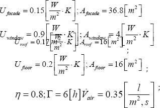
Where, ρ_air ,C_air , and V_ajr , are the density [kg/m3], capacity [J/(K.kg)] and volume flow [l/(s, floor area)] of the ventilation air, respectively. η is the efficiency of the ventilation heat exchanger and A_floor is the floor area. Since the building has a ventilation system with heat recovery, the tightness should be very high; therefore, the air leakage assumed to be almost zero. ∑u-a is the sum of the heat transfer coefficient [W/(m².K)] multiplied by the heat transfer area [m²] for different parts of the building envelope.

The time constant [h] of a building can be written as [9]:

Since the experimental data for the radiator power was approximately 660 [W] at maximum capacity, the data for the building model was adjusted reasonably to this value. The time constant for the simulated building was estimated at 6 hours. The following data were used in the simulations:

With these values, the heat capacity, C, of the building (including envelope and air) is 353 890 [J/K]. This value has been used in Simulink models. Note that the above values have been selected in consideration of the maximum capacity of the radiator, which explains the choice of the very low time constant as it corresponds to a very light house [9].

Results

Figure 3 shows the experimental setup used to obtain the step response for the radiator and the input power to the radiator (supply power as shown in equation 1).

The supply water for the radiator was heated using a heat exchanger (VVX), and the flow to the radiator was controlled by valve V1 and bypass BP1. At the start of each experiment, the overall temperature was 21 °C, and during the heating process, until the desired supply temperature was reached, BP1 was opened and V1 was closed. When the water temperature reached the desired level, V1 opened and B P1 closed.

When measuring the step response from the radiator, it was important to see how the power supplied to the radiator was affected by various volume flows. To calculate the supplied power using equation 1, the temperatures of the water to and from the radiator (supply and return temperatures) and the volume flow through the system were measured. Figure 4 shows how the power supplied to the radiator (equation 1) changes over time for different volume flows.

When a steady state is attained for each flow, the difference in supply power between different volume flows is small. The supply power was calculated using equation 1.

To obtain the step responses at different volume flows, the power emitted from the radiator must be calculated. This was done by measuring the surface temperature of the radiator and the room temperature and using equation 4, where the power supplied at steady state, , for various volume flows was obtained according to Figure 4.

Figure 5 shows that with higher mass flow, the step response becomes shorter and the emitted power increases. The steady state emitted power from the radiator at different volume flows can be seen in Figure 4 & 5. Figure 6 shows the steady state power emitted from the radiator for various volume flows after data fitting. The relation between and based on experimental data after data fitting is (equation (11) and Figure 6):

Based on Figure 5, the time constant for emitted power, i.e., the time to reach 63% of the final value, can be plotted for different volume flows, as shown in Figure 7. The obtained relation between the time constant of the radiator, and based on the experimental data after data fitting is (see equation (12) and Figure 7):

A simplified overall model for TRVs is shown in Figure 8, and a sub-model of the building model in Simulink is shown in Figure 9. Additional Simulink models are shown in the Appendix.

The output signal of the controller in Figure 8 is a new value for the steady state radiator power, which in turn determines the mass flow and the time constant of the radiator. When the time constant and the steady state value of the emitted power from the radiator are calculated, the emitted power, including the time constant, will be determined. This is a new way of thinking concerning building a model of hydronic radiators and controlling them.

The results of simulations for four different cases can be seen in Figures 10-13. The simulation time is 48 hours. In all cases, the internal power gain (heat from people, electrical appliances, etc.) alternates from 0 to 200 [W] periodically every 4 hours. The outdoor temperature also varies sinusoidally between -5 and 5 ஺C with a period of 24 [h]. The total emitted heat from radiators was integrated during 24 hours to calculate the energy use. Figure 10, 11 show the results of simulations where a well- functioning TRV is used. Figure 10 shows the results of the simulation when a PI controller is used. The gain and the integral time are 0.19 and 10x10-5, respectively. Figure 11 shows the result of simulations where a P controller with gain of 0.5 and a P-band of 2 ஺C is used. As many TRVs malfunction, two cases with poorly functioning TRVs have been simulated. The results of the malfunctioning TRVs are shown in Figures 12, 13. In some cases, they do not open or close fully, resulting in a low indoor temperature or energy waste.

As shown in Figure 10, a PI controller produces very small indoor-temperature fluctuations (approximately 1 ºC) around the set point (21 "C).

As shown in Figure 11, a P controller produces very small indoor-temperature fluctuations (1 ºC) around the set point (21 "C). However, there is always residual error that cannot be eliminated.

As shown in Figure 12, the mass flow varies between 2x10-3 and 5.2x10-3 [kg/s], which means that the TRV is never closed. Such errors unfortunately occur in some TRVs and lead to high temperatures and energy waste.

As shown in Figure 12, the mass flow varies between 9.20x10-4 and 2.42x10-3 [kg/s], which means that the TRV does not open fully, resulting in very low indoor temperature.

In some cases, where the fluctuations are very high because of a malfunctioning TRV, a higher set point must be chosen to not undercut the minimum indoor temperature (Figure 13). These results in a waste of energy compared to a well-functioning TRV, as shown in Figure 14.

Discussion and Conclusion

The development of a model of a hydronic radiator to investigate different control strategies in buildings has not been extensively researched in previous studies. The key to the investigation is to build a combined "black box" and physical model, where the hot water mass flow is used as the input signal and the heat emitted from radiator is the output signal. The temperature of the hot water is varied by central heating system as a function of the outdoor temperature and cannot be affected by individual buildings. This is the way that the heat from radiators is controlled in most buildings in Sweden.

The results of simulations in this paper suggest that the temperature control of the studied building will be improved by using a well-functioning TRV instead of a malfunctioning TRV. In the developed Simulink model, different control strategies can be investigated. The smaller fluctuations of the indoor temperature when using the well-functioning TRV rather than a malfunctioning TRV result in a better indoor climate. Different types of TRV failures may produce large indoor-temperature oscillations, very high/very low indoor temperature and/or high energy use. In some cases, a poor-functioning TRV results in unreasonably high indoor temperatures with high energy use, whereas in other cases, it might cause a very low indoor temperature. However, the difference between well-functioning controllers (P and PI) is marginal.

Limitations and Error Sources

a. Different volume flows were tested in duplicate. The average of the two runs was then used to avoid error. However, the result could have been different if more runs for each volume flow were tested.

b. Another limitation was that the simulations were only run over 48 hours and not throughout a whole year.

c. The results from the experiment are applicable only to the radiator used in the experiment (Purno C11-compact), different radiators would likely have different responses.

d. The room in which the experiment was conducted had specific interior and technical equipment that could influence the heat transfer process; therefore, the results are limited to the specific room.

e. The experiment was conducted until the surface temperature of the radiator was constant and had reached a steady state. However, after some time, it was concluded that the system had reached steady state even though the temperature was not completely constant. Had the experiment been run for a longer time, the steady state of the emitted effect may have been slightly higher.

f. The room temperature varied depending on when the experiment was conducted. This was particularly noticeable for subsequent tests as the ambient temperature was slightly higher due to previous tests. This mainly affects the emitted effect.

g. The experiment was monitored by measuring devices that were connected to sensors around the radiator. The volume flow sensor has a stated margin of error of a few percent, making it the largest source of error from the equipment.

h. One of the focuses of the experiment was to keep the secondary system as a closed system to maintain the same amount of water in the system for all the experiments. However, there was a small leak that allowed water to escape. Moreover, air bubbles entered the system. Between each test, the secondary system was refilled. The amount of water could therefore differ from the previous test.

i. Rust inside the radiator could also affect the heat transfer process, partly by affecting the volume flow, but the coating could also serve as an extra insulator and thus slow the heat output in the form of conduction.

j. When the temperature in the system increases, so does the pressure. To reduce the impact this change would have on the volume flow, a speed-controlled pump was used. This pump did not fully compensate for this problem, which led to the volume flow changing slightly during the heating process.

k. The temperature of the water supplied to the heat exchanger during the test changed. After a few minutes, there was a dip in the temperature of the system, which had an impact on the induced, and thus the emitted, effect.

References

- Pérez-Lombard L, Ortiz J, Pout C (2008) A Review on Buildings Energy Consumption Information. Energy and Buildings 40(3): 394-398.
- Soleimani-Mohseni M (2005) Modelling and Intelligent Climate Control of Buildings. Chalmers University of Technology, Dept. of Energy and Environment, Gothenburg, Sweden.
- Tahersima F (2011) Eliminating Oscillations in TRV-Controlled Hydronic Radiators. 50th IEEE Conference on Decision and Control and European Control Conference (CDC-ECC), Orlando, FL, USA.
- Soleimani-Mohseni M (2002) Intelligent thermostats save energy and give improved control performance. ACEEE Summer Study on Energy Efficiency in Buildings. Panel 7: Information and Electronic Technologies: Promises and Pitfalls, Monterey, USA.
- Ruiz Calvo P (2014) Research about energy performance of low-flow radiator systems. University of Gavle, Sweden.
- Kyu NR, Myoung SY, Kwang WK (2011) Evaluation of the control performance of hydronic radiant heating systems based on the emulation using hardware-in-the-loop simulation. Building and Environment 46(10): 2012-2022.
- Soleimani-Mohseni M, Backstrom L, Eklund R (2012) EnBe- Energiberakningar, Studentlitteratur, ISBN: 9789144088693 in Swedish.
- Thomas B (2016) Modern Reglerteknik, Liber, ISBN: 9789147112128 in Swedish.
- Abel E, Elmroth A, Byggnaden som system, Studentlitteratur (2016) ISBN 9789144115887 in Swedish.